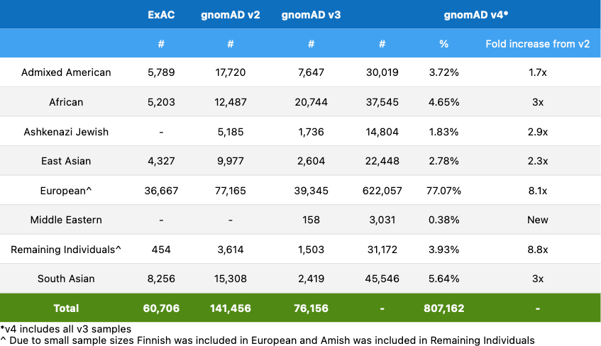
Today, we are delighted to announce the release of gnomAD v4, which includes data from 807,162 total individuals. This release is nearly 5x larger than the combined v2/v3 releases and consists of two callsets: exome sequencing data from 730,947 individuals, including 416,555 individuals from the UK Biobank, and genome sequencing data from 76,215 individuals. Both callsets within v4 were aligned to build GRCh38 of the human reference genome.
The gnomAD v4 release adds additional global diversity and includes ~138,000 individuals of non-European genetic ancestry. However, the new inclusion of cohorts such as the UK Biobank means that the proportion of samples with European ancestry is higher than in previous releases. The genetic ancestry group breakdown of gnomAD v4 is:
In this blog post, we will cover important updates from gnomAD v2/v3, how we created gnomAD v4, and details of the quality control (QC) done on gnomAD v4.
Updates in gnomAD v4
Genetic ancestry updates
All of the members of the gnomAD project continue to discuss best approaches to defining genetic ancestry across the gnomAD dataset. We have made a few terminology updates in this release based on feedback from the community. For more information see: https://gnomad.broadinstitute.org/news/2023-11-genetic-ancestry.
Minimum Viable Product (MVP)
In the v4 release, we have moved towards the model of incremental releases. This means that the v4.0 release is a minimum viable product (MVP) release, or a release that contains only the most critical components of the gnomAD database. This means that the v4.0 release will not have all of the features of the v2 or v3 releases, and these features will be released in subsequent minor releases. This includes gene constraint, proportion expressed across transcripts (pext) scores, sub-genetic ancestry groups, variant co-occurrence, and regional missense constraint. To see a full list of features not included in v4 MVP and where to access them in past versions, please see this FAQ.
Differences between gnomAD v3 and v4
The 76,156 genomes from gnomAD v3.1.2 have been included in gnomAD v4. We have not updated the quality control (QC) of these samples, but we have updated some of the frequencies within the HGDP and 1000 Genomes (HGDP/1KG) subset.
HGDP/1KG genetic ancestry group updates + subset frequencies
We are invested in following the current best practices in defining and labeling genetic ancestry within gnomAD. As part of the v4 release, we have updated the genetic ancestry group labels within the HGDP/1KG subset to follow updated guidance from Anders et al (2020):
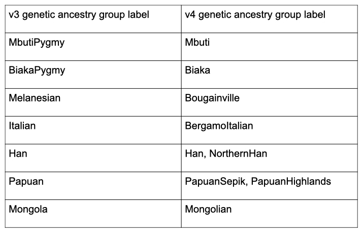
In addition to updating the genetic ancestry group labels within the HGDP/1KG subset, we have also updated the sample filtering within this subset as part of the v4 release. We have updated the relatedness filtering within this subset and removed one additional PCA outlier sample following the guidance of Zan Koenig et al. The sample counts are summarized in the table below:
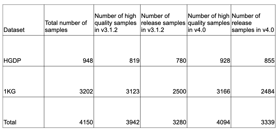
Because we have updated the sample filtering criteria for the HGDP/1KG subset, we have also updated the allele frequency information for these samples. This information is available in the gnomAD v4 display and within the gnomAD v4 files listed on the Downloads page.
Subsets
One major difference between gnomAD v3 and v4 is the number of subsets included in each release. The gnomAD v3 release had five subsets, whereas gnomAD v4 has a single subset (non-UKBB; see Dataset selection). Note that the v4 subset is not displayed on the browser, but frequencies for this subset are available for download in our downloadable files.
We have removed support for subsets from the gnomAD v4 exomes for two major reasons: given the large size of gnomAD v4 and the small size of any single cohort, we do not feel that the prevalence of any disease is high enough to warrant subsets. In addition, there is increased inclusion of biobank samples, and we do not have concise phenotype metadata for these and many other gnomAD samples, so we cannot ensure that samples in a non-disease subset do not have the specified disease.
Updated filtering allele frequency
We have released a new, combined filtering allele frequency (FAF), which integrates variant frequencies across the 730,947 exomes and 76,215 genomes. The exome FAF and genome FAF are still listed on the variant pages as well.
Structural Variants
We have generated copy number variant and structural variant calls on the v4 exomes and genomes, respectively. For more information, see:
- Exome CNVs: https://gnomad.broadinstitute.org/news/2023-11-v4-copy-number-variants
- Genome SVs: https://gnomad.broadinstitute.org/news/2023-11-v4-structural-variants
Variant annotations
We have updated the following variant annotations to help users interpret the clinical and functional effects of variants without needing to navigate to other resources:
- REVEL
- CADD
- phyloP
- spliceAI
- Pangolin
We would particularly like to thank Kevin Kazmierczak, Laure Fresard, Alex Wahl, Alex Colavin, Naomi Fox, and Keith Nykamp at Invitae for their assistance in generating Pangolin annotations and Kishore Jaganathan and Kyle Farh at Illumina for their assistance in generating SpliceAI annotations
We have also incorporated Global Alliance for Genomics and Health (GA4GH) Variant Representation Specification (VRS) annotations in this release. For more information, please see our blog post.
Creating gnomAD v4
This section and the two sections below (sample and variant QC) describe how we generated the v4 exomes callset. For more information about the v4 genomes, see previous blog posts (v3, v3.1, v3.1.2)
The full gnomAD v4 exomes dataset, like the gnomAD v4 genomes, was created by combining all samples’ genomic VCFs (gVCF) into a single dataset using Hail. The v4 exomes callset is stored as a VariantDataset (VDS), Hail’s newest implementation of the scalable variant call representation (SVCR) data structure. To create our release containing 730,947 samples, we actually processed over 955,000 samples, and the scalability of the VDS format means that the full v4 dataset (955,213 samples) only uses 18TB in storage (vs 897TB for a traditional project VCF)
Interval QC
Due to the lossless conversion of gVCF to VDS, the gnomAD v4 exomes callset contains every observed variant and reference block start from each sample’s gVCF. To determine which intervals had adequate coverage (and were therefore appropriate for QC), we added a new step to the beginning of our QC pipeline: interval QC. In this step, we calculated coverage per exome calling interval for each sample. We assessed intervals with a padding of 50 base pairs from the Broad’s exome calling interval list and the UK Biobank’s exome calling intervals. Intervals where 85% of all samples had a mean coverage of at least 20X were considered high coverage intervals.
High quality sites definition
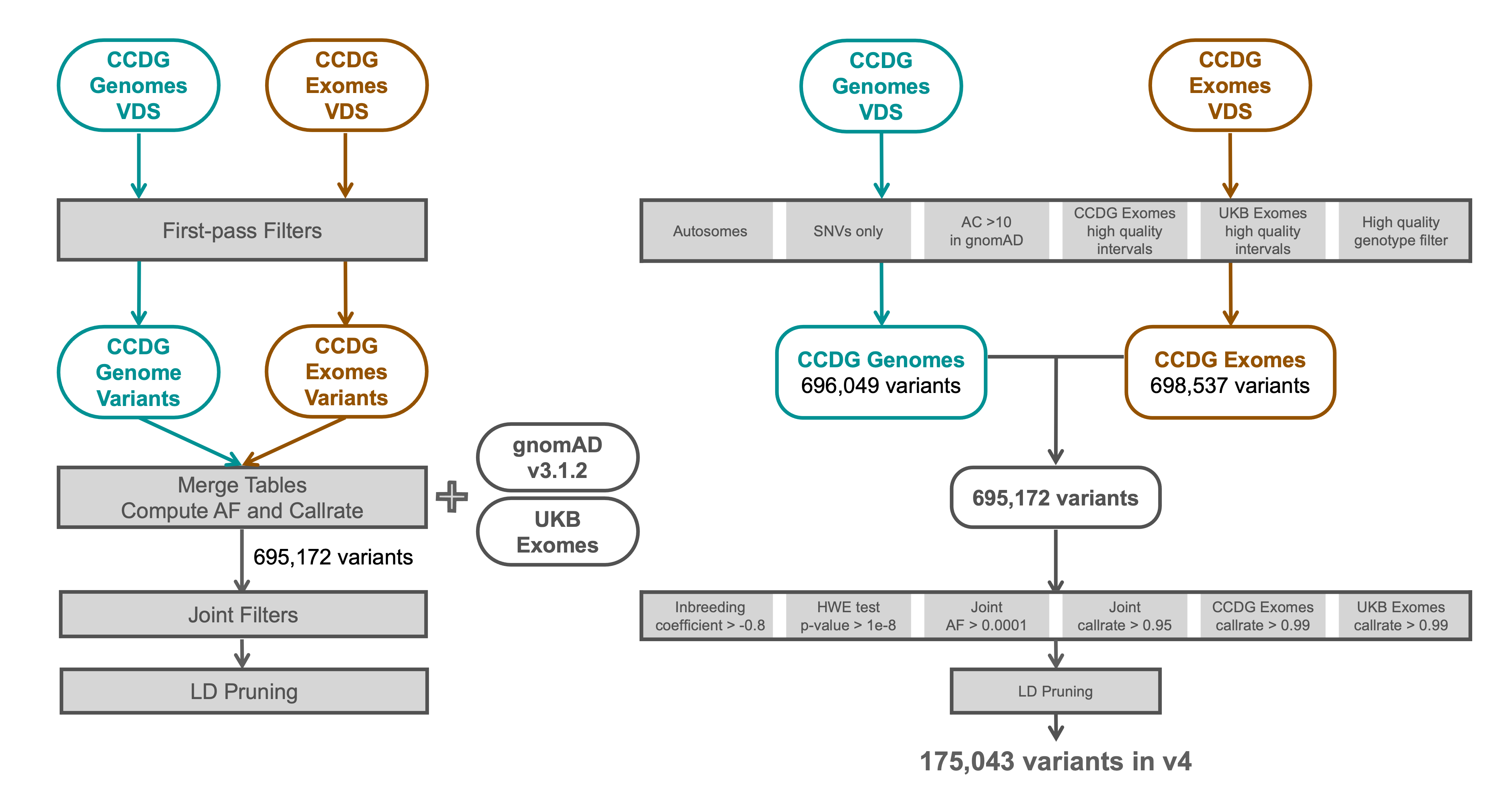
We defined a set of high quality sites on which to perform specific steps of sample QC, including relatedness and genetic ancestry inference. We selected autosomal, biallelic, single nucleotide variants (SNVs) from the following datasets:
- gnomAD v3
- Centers for Common Disease Genomics (CCDG) exomes and genomes
- UK Biobank (UKB) exomes
We selected variants within high-quality intervals of both the CCDG and UKB exomes data with allele counts (AC) > 10 in gnomAD v3 that also passed high quality genotype filters in the CCDG exome and genome data. We then filtered to variants with an allele frequency (AF) > 0.0001, inbreeding coefficient > -0.8, HWE pvalue > 1e-8, and a call rate > 95% in the combined set of gnomAD v3 and CCDG genome data, plus a call rate > 99% in both the CCDG and UKB exomes. Finally, we LD-pruned the variants, which left a total of 175,043 sites.
Sample QC
The biggest challenge to creating the gnomAD v4 release was updating our sample quality control (QC) methods to efficiently compute at this scale and level of data heterogeneity: the 955,000 exomes processed in this release were inferred to span 20 different exome capture platforms. The areas where we added the biggest improvements were contamination estimation, relatedness inference, and sample outlier detection.
The major steps taken in v4 sample QC are listed here (with details following):
- Samples with obviously bad quality were removed using hard filters
- We inferred exome capture platform for each sample
- We inferred sex karyotypes for each sample using normalized sex chromosome coverage
- We inferred relatedness between samples, including between the v4 exomes and genomes, and identified pairs of first and second degree relatives
- We used genetic similarity to cluster and identify genetic ancestry groups
- We filtered samples based on QC metrics
Hard filters
One major step to creating any gnomAD release involves the importing and merging of study-provided and read-based sample metadata. When creating the v4 release, we found that a large number of samples were missing read-based QC metadata, including contamination estimates. To remove samples with evidence of contamination, we applied the novel metric Contamination from Homozygous Alternate Reference Reads (CHARR) to estimate contamination from the v4 genotype data rather than needing to recompute over the raw read data. This enabled us to estimate contamination at a fraction of the time and cost (~$0.0003/sample) as compared to traditional methods.
In addition to contamination, we computed sample QC metrics using the Hail sample QC module on all autosomal, biallelic SNVs. In summary, the hard filtering step removed samples that were outliers for the following metrics:
- Contamination (mean AB biallelic SNPs) > 1.5%
- Number of singletons > 5000
- Heterozygous: homozygous ratio > 10
- Bases with DP over 1X < 5x10⁷
- Bases with DP over 20X < 4x10⁷
- Proportion chimera > 0.05
- Mean chromosome 20 DP < 10X
- Callrate calculated over high quality sites < 0.8
Platform inference
Because the sample QC metrics vary based on the sequencing platform, we ran platform inference on the gnomAD v4 samples. We performed a principal components analysis (PCA) using missingness rate calculated per sample for each exome calling interval (intersection of Broad and UK Biobank intervals). Using nine principal components (PCs), we inferred that there are 20 unique exome sequencing platforms in gnomAD v4.
Sex inference
Similar to gnomAD v3, we used normalized sex chromosome coverage to infer sex. We used Hail’s impute_sex_chromosome_ploidy module to calculate mean coverage across chromosomes X (chrX) and Y (chrY). For chrX, we calculated mean depth across variants in non-pseudoautosomal (non-PAR) regions, and we excluded variants falling within low-complexity and segmental duplication regions. For chrY, we calculated mean depth across all reference blocks in non-PAR regions. We then normalized the mean chrX and chrY coverage using mean coverage across chromosome 20 to estimate chrX and chrY ploidy.
Due to the heterogeneity of the data across different sequencing platforms, we computed sex karyotype cutoffs per platform. We fit Gaussian mixture models per platform for chrX and chrY ploidy using two components. Samples assigned to the cluster with lower mean chrX ploidy cluster relative ploidy were assigned a chrX ploidy of “X” (single copy of chrX), and samples assigned to the higher mean cluster were assigned “XX” (two copies of chrX). The same process was taken to assign samples to "" (zero copies of chrY) and “Y” (single copy of chrY) karyotypes. We then combined these two karyotypes, which led to the following combinations of sex karyotypes: X, XX, XY, and XXY
We then calculated the mean and standard deviation of XX and XY ploidy distributions to determine cutoffs for sex aneuploidies, and we calculated the fraction of homozygous alternate genotypes per sample on chrX to inform sex karyotype adjustment for samples inferred to have sex karyotypes of X0. The final list of possible sex karyotypes is: X, XX, XXX, XXXY, XXY, XXYY, XY, XYY, and ambiguous.
Relatedness inference
Computing relatedness between samples was the most complex computational challenge within gnomAD v4 sample QC. To determine pairs of first and second degree related samples in the dataset, and to ensure no overlap between the exomes and genomes, we needed to compare over one millionsamples in a pairwise manner, effectively requiring the computation of a one million by one million matrix. We were not confident that our previous tool, Hail’s pc_relate module, would be able to complete this computation. To solve this problem, we used a CUDA-based implementation of KING (cuKING; implemented by Leonhard Gruenschloss) to compute pairwise relatedness across the gnomAD v4 exomes and genomes. cuKING was able to compute relatedness across the v4 exomes and genomes in approximately 1.5 hours at a cost of $243.
Once we inferred pairs of first and second degree related samples, we used Hail’s maximal_independent_set module to the minimum number of samples required to release a dataset with completely unrelated individuals. When multiple samples were selected, we prioritized releasable samples in the v4 genomes, then v4 exome samples over unreleasable genome samples, then samples with higher mean coverage across chromosome 20.
Genetic ancestry inference
The method we used to infer genetic ancestry was similar to the method used in v3 and v3.1. We ran a PCA using Hail’s hwe_normalized_pca module to cluster samples based on their genetic similarity and computed 30 PCs over the 175,043 previously defined high quality sites (see High quality sites definition). We then visually inspected the PCs and generated precision-recall curves to determine which PCs were capturing variance explained by our known ancestry descriptors (see our Genetic ancestry blog post for more details about these labels). We determined that the first 20 PCs captured most of the variance and trained a random forest (RF) classifier using those 20 PCs as features on samples with known ancestry descriptors. Samples with the following probability of group assignments were assigned to the relevant labels:
- AFR: 0.93
- AMR: 0.86
- ASJ: 0.88
- EAS: 0.96
- FIN: 0.91
- MID: 0.56
- NFE: 0.78
- SAS: 0.96
Any samples that we were unable to cluster using these probabilities were grouped into “Remaining individuals”. The probability cutoffs were determined by holding back 20% of the samples with known ancestry descriptors for evaluation of the model. Note that the genetic ancestry groups within gnomAD are artificially created and not naturally occurring groups.
QC metrics outlier filtering
In gnomAD v3.1.2, we discovered that our previous method of sample QC metrics outlier filtering was inadvertently removing highly diverse samples. To prevent this from occurring in v4 and future releases, we updated our method of sample QC metrics outlier filtering. In this release, we combined two approaches to sample outlier detection to create an ensemble approach. The two approaches were:
- Platform stratification + genetic ancestry PC regression filtering: We first stratified sample QC metrics distributions per inferred exome sequencing platform, and then we regressed out the 20 PCs computed during the genetic ancestry inference PCA. This method, adapted from the method used in v3, allowed us to treat genetic ancestry as continuous, rather than requiring us to stratify samples by their discrete genetic ancestry group.
- 50 nearest neighbors: We calculated sample QC metrics distributions based on a sample’s 50 nearest neighbors. Nearest neighbors were determined per platform, and Euclidean distances were computed using the 20 PCs computed in the genetic ancestry PCA
For both of these methods, we compared samples to the defined distribution and flagged any samples for filtering if the sample’s value was 4 median absolute deviations (MADs):
- over or under the following metrics
- insertion : deletion ratio
- transition : transversion ratio
- singleton transition : transversion ratio
- We only computed this metric for samples with:
- 50 nearest neighbors:
- number of singletons > median number of singletons calculated with the 50 nearest neighbors
- Platform stratification + genetic ancestry PC regression filtering: * residual number of singletons > median residual number of singletons for that platform
- 50 nearest neighbors:
- We only computed this metric for samples with:
- OR over the median for:
- heterozygous : homozygous ratio
Only samples that were filtered by both the 50 nearest neighbors and the platform stratification + genetic ancestry PC regression filtering were removed.
Variant QC
Similar to gnomAD v3, we computed our variant QC metrics in Hail and used the allele-specific (AS) version of GATK Variant Quality Score Recalibration (VQSR) to compute a score indicating the confidence that a variant is real vs an artifact. We used the following features:
- SNVs: AS_FS, AS_ReadPosRankSum, AS_MQRankSum, AS_QD, AS_MQ
- indels: SNVs: AS_FS, AS_ReadPosRankSum, AS_MQRankSum, AS_QD
To train our AS-VQSR model, we used the GATK bundle training resources (hapmap, omni, 1000 genomes, mills indels) and ~48,000 transmitted singletons (alleles confidently observed exactly twice in the gnomAD dataset, once in a parent and once in a child) and ~12,500 sibling singletons (alleles confidently observed exactly twice in gnomAD in two siblings) from 12,731 trios and 26,738 sibling pairs present in our raw data, respectively.
We evaluated the results of our VQSR filtering by assessing performance in the same metrics used for v2 and v3: de novo looking mutations in our 12,731 trios, Ti/Tv ratio, proportion singletons, proportion biallelic variants, variants in ClinVar, and precision and recall in two truth samples present in our data: NA12878 and a pseudo-diploid sample (a mixture of DNA (est. 50.7% / 49.3%) from two haploid CHM cell lines) for which we have good truth data.
The figure below illustrates the performance of our VQSR filtering on NA12878.
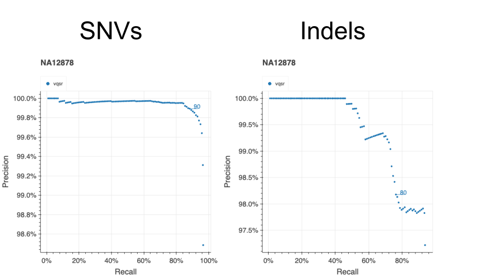
This model filtered 15.2% of SNVs and 29.0% of indels.
In addition to VQSR, we also applied the following hard filters:
- AC0: No sample had a high quality genotype at this variant site (GQ>=20, DP>=10 and allele balance > 0.2 for heterozygotes)
- InbreedingCoeff: there was an excess of heterozygotes at the site compared to Hardy-Weinberg expectations using a threshold of -0.3 on the InbreedingCoefficient metric.
62,901,592 SNVs and 6,189,261 indels pass all filters in the v4 release.
Acknowledgments
We want to thank a few specific people for their critical contributions to the v4.0 release while also acknowledging the wide network of individuals required to make gnomAD possible.
First, as always, we are incredibly grateful to the 308 data contributors who allowed their data to be used in this project. The gnomAD project would not be possible without their contributions.
Christine Stevens, Sinéad Chapman, Caroline Cusick, and Sam Baxter were critical in sifting through the mountain of sample metadata required to produce v4. Charlotte Tolonen, Sam Bryant, and Sam Novod played important roles in data generation, and Grace Tiao’s leadership and guidance helped get v4 production started.
Julia Goodrich single-handedly kept the v4.0 release timeline in check and played an enormous role in QC. Kristen Laricchia and Mike Wilson were also critical to production, each taking ownership of key QC steps, and both contributed particularly immense amounts of brainpower to thorough code review. Wenhan Lu was crucial in determining our set of high quality sites and in calculating sample contamination. Leonhard Gruenschloss and Vlad Saveylev were instrumental to solving our relatedness inference problem and allowed us to compute our 1 million x 1 million pairwise relatedness with ease. Laura Gauthier, Sam Lee, and Lee Lichtenstein helped the team make sense of numerous variant quality metrics and proceed with variant QC. Daniel Marten helped tremendously with building and applying models for variant QC, and Qin He contributed critical efforts to updating our variant annotations.
Tim Poterba, Chris Vittal, and Dan King went above and beyond to support the production team during QC efforts. They deserve a massive thank you for their patience as we broke Hail and for their tireless efforts to help ensure our huge computations ran to completion. Jackie Goldstein and Daniel Goldstein’s support with Hail Batch was critical to getting VRS variant annotations into v4.
Jack Fu, Isaac Wong, Ryan Collins, Cal Liao, Daniel Ben-Isvy, and Lily Wang generated and QC’ed the v4 exome copy number variant dataset. Xuefang Zhao, Ryan Collins, Mark Walker, Chris Whelan, and Nehir Kurtas produced and assessed the v4 genome structural variant dataset. We want to thank Harrison Brand in particular for his leadership and guidance around both the genomes SV and exomes CNV datasets.
Matt Solomonson, Riley Grant, Phil Darnowsky, Ben Weisburd, and Steve Jahl did the work of loading the v4 release into the gnomAD browser and making necessary updates to the browser and website, ensuring our data is easily accessible and understood by all.
Finally, thanks to critical guidance by members of the gnomAD steering committee and all of the staff who contributed their effort across the Broad, including the compliance team – gnomAD is truly the result of a massive collaboration!
References/links
- Lu, W., Gauthier, L.D., Poterba, T., Giacopuzzi, E., Goodrich, J.K., Steves, C.R., King, D., Daly, M.J., Neale, B.M. & Karczewski, K.J. CHARR efficiently estimates contamination from DNA sequencing data. bioRxiv 2023.06.28.545801 (2023). https://doi.org/10.1101/2023.06.28.545801
- Koenig, Z., Yohannes, M.T., Nkambule, L.LGoodrich, J.K., Kim, H.A., Zhao, X., Wilson, M.W., Tiao, G., Hao, S.P., Sahakian, N., Chao, K.R., gnomAD Project Consortium, Talkowski, M.E., Daly, M.J., Brand, H., Karczewski, K.J., Atkinson, E.G. & Martin, A.R. A harmonized public resource of deeply sequenced diverse human genomes. bioRxiv 2023.01.23.525248 (2023). https://doi.org/10.1101/2023.01.23.525248
- Bergström, A., McCarthy, S. A., Hui, R., Almarri, M. A., Ayub, Q., Danecek, P., Chen, Y., Felkel, S., Hallast, P., Kamm, J., Blanché, H., Deleuze, J. F., Cann, H., Mallick, S., Reich, D., Sandhu, M. S., Skoglund, P., Scally, A., Xue, Y., Durbin, R., … Tyler-Smith, C. (2020). Insights into human genetic variation and population history from 929 diverse genomes. Science (New York, N.Y.), 367(6484), eaay5012. https://doi.org/10.1126/science.aay5012
Updated in August 2025 to fix typo and formatting.