Originally published on the MacArthur Lab blog.
We are thrilled to announce the release of gnomAD v3, a catalog containing 602M SNVs and 105M indels based on the whole-genome sequencing of 71,702 samples mapped to the GRCh38 build of the human reference genome. By increasing the number of whole genomes almost 5-fold from gnomAD v2.1, this release represents a massive leap in analysis power for anyone interested in non-coding regions of the genome or in coding regions poorly captured by exome sequencing.
In addition, gnomAD v3 adds new diversity – for instance, by almost doubling the number of African American samples we had in gnomAD v2 (exomes and genomes combined), and also including our first set of allele frequencies for the Amish population.
Here’s the population breakdown in this release:
| Population | Description | Genomes |
|---|---|---|
| afr | African/African American | 21,042 |
| ami | Amish | 450 |
| amr | Latino/Admixed American | 6,835 |
| asj | Ashkenazi Jewish | 1,662 |
| eas | East Asian | 1,567 |
| fin | Finnish | 5,244 |
| nfe | Non-Finnish European | 32,299 |
| sas | South Asian | 1,526 |
| oth | Other (population not assigned) | 1,077 |
| Total | 71,702 |
In this blog post we wanted to lay out how we generated this new data set, specifically:
- A new method, implemented in Hail, that allows the joint genotyping of tens of thousands of whole genomes
- The approach we took for quality control and filtering of samples
- The approach we took for quality control and filtering of variants
But first we’d like to say thanks to the many, many people who made this release possible. First, the 141 members of the gnomAD consortium – principal investigators from around the world who have generously shared their exome and genome data with the gnomAD team and the scientific community. Their commitment to open and collaborative science is at the core of gnomAD; this resource would not exist without them. And of course, we would like to thank the hundreds of thousands of research participants whose data are included in gnomAD for their dedication to science.
The Broad Institute’s Genomics Platform sequenced over 80% of the genomes of this gnomAD release. We thank them for this important contribution to gnomAD, and for storage and computing resources essential to the project. The Broad’s Data Sciences Platform also played a crucial role – the Data Gen team for producing the uniform gvcfs required for joint calling, and Eric Banks and Laura Gauthier for their work on the immense callset that forms the core of gnomAD. We also owe an enormous debt of gratitude to the Hail team, especially Chris Vittal, for creating the novel gvcf combiner described below; a callset of this scale would have been impossible without his engineering.
Konrad Karczewski, Laura Gauthier, Grace Tiao and Mike Wilson made absolutely critical contributions to the quality control and analysis process. In addition, the Broad’s Office of Research Subject Protection were key contributors to the management of gnomAD’s regulatory compliance.
The amazing gnomAD browser is the creation of Nick Watts and Matt Solomonson, and there was considerable work required for this version to scale to the size of this dataset and move all of our annotations onto GRCh38. And finally, we wanted to thank Jessica Alföldi, who has contributed in myriad ways to the development of this resource, including a critical role in communicating with principal investigators, assembling the sample list, and gathering the permissions required for this release to be possible.
Calling short variants in tens of thousands of genomes
A major challenge we had to overcome when putting together gnomAD v3 was how to handle the massive increase in data from gnomAD v2. Getting to the point of having over 70,000 releasable samples actually required making a call set that spanned nearly 150,000, from which we removed samples that failed our various quality filters, were related to other samples, belonged to individuals with pediatric disease or their first-degree relatives, or didn’t have appropriate permissions for data release.
Our previous strategy for gnomAD v2 involved joint-calling all samples together using GenomicsDB and GATK GenotypeGVCFs to produce a VCF file with a genotype for each sample at every position where at least one sample contains a non-reference allele. This approach required too much time and memory to run reliably without errors or failures when using the number of samples present in gnomAD v3. Even if it had scaled, the output would have been a dense, multi-sample VCF for all 150,000 samples, which would have been about 900TB in size and prohibitively expensive to store and compute over.
Instead, Chris Vittal and Cotton Seed in the Hail team took on the challenge of ingesting the samples’ genomic VCFs (GVCFs) directly in Hail in order to expose all samples’ genotypes together for our analyses. GVCFs are generated for each sample separately and they contain one row for each genomic position where a non-reference allele was found in the sample and, unlike VCFs, a row for each reference block start. Reference blocks are contiguous bases where the sample is homozygous reference within certain confidence boundaries. In our case, we used the following three confidence bins:
- No coverage / evidence
- Genotype quality < Q20
- Genotype quality >= Q20
For each of these bins, the reference block stores the minimum and median coverage, and the minimum genotype quality for the bases comprised in the block.
One of the major challenges in putting these data together is to align the non-reference genotypes and the reference blocks from the different samples for each chromosome/position. This was achieved by computing an efficient partitioning of the genomes that can be used for all samples and by combining the GVCFs using a tree approach.
The resulting data is a matrix of genomic positions and samples, where a row is present for each position where either a sample is non-reference or a reference block starts in any sample. The information about reference genotypes is only present at the beginning of each reference block (which can spend thousands or even tens of thousands of bases), making the representation sparse.
Using this new sparse data format, gnomAD v3 only takes up 20TB (45x less than using the previous dense format!). This new format scales linearly with the number of samples and is lossless with respect to the input sample GVCFs, which has the following important implications:
- Much more granular QC metrics are preserved at each non-reference genotype in the data, such as strand balance, read and base quality ranksum, etc.
- New data can be appended to existing data without re-processing of the existing samples, solving the famous “N+1” problem
- While not yet implemented, it should be possible to re-export a GVCF from this format, removing the need for storing GVCFs.
Sample QC
The overall sample QC process we used for gnomAD v3 was similar to that of v2.1, with a few changes and improvements along the way. The main improvements are the use of normalized coverage on both X and Y in order to infer sample sex, and a new way of filering outliers based on QC metrics.
Our sample QC process can be summarized as:
- Hard filters were applied to eliminate samples of obviously bad quality
- We inferred sex for each sample and removed samples with sex chromosome aneuploidies or ambiguous sex assignment.
- We defined a set of high quality sites on which to compute relatedness and ancestry assignment
- We inferred relatedness between samples, and identified pairs of 1st and 2nd degree relatives, allowing us to filter to a set of unrelated individuals
- We assigned ancestry to each sample
- We filtered samples based on QC metrics
Hard filtering
We computed sample QC metrics using the Hail sample_qc
module on all autosomal bi-allelic SNVs. We removed samples that were clear outliers for:
- n_snps: n_snp < 2.4M or n_snp > 3.75M
- n_singleton: n_singleton > 100k
- r_het_hom_var: r_het_hom_var > 3.3
In addition, we removed all samples with a mean coverage < 18X.
Sex inference
To impute sex, we computed the mean coverage on non-pseudoautosomal (non-PAR) regions of chromosome
X and Y and normalized these values using the mean coverage on chromosome 20. In addition, we ran
Hail impute_sex
function on the non-PAR regions of chromosome X to compute the inbreeding coefficient F. Based on
these three metrics we assigned sex as follows:
- Males:
- chromosome X (non-PAR) F-stat > 0.2 &
- 0.5 < normalized X coverage > 1.4 &
- 1.2 < normalized Y coverage > 0.15
- Females:
- chromosome X (non-PAR) F-stat < -0.2 &
- 1.4 < normalized X coverage > 2.25 &
- normalized X coverage < 0.1
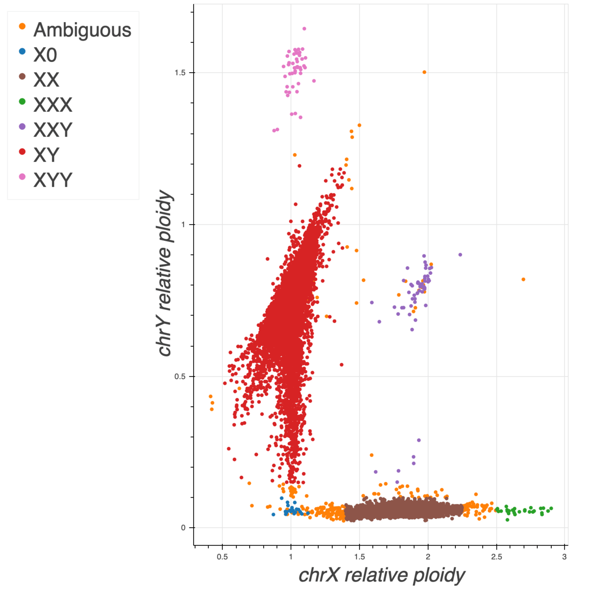
Note that the finger pointing down from the males cluster is likely due to mosaic loss of Y in older males as it correlates with sample age.
Defining a high quality set of sites for QC
In order to perform relatedness and ancestry inference, we first selected a set of high quality QC sites as follows:
- We took all sites that were used for gnomAD v2.1 and lifted them over to GRCh38
- We added 5k sites that were curated by Shaun Purcell when performing GWAS and lifted these sites over
- From these two sets of sites, we then selected all bi-allelic SNVs with an Inbreeding coefficient > -0.25 (no excess of heterozygotes)
In total, we ended up with 94,148 high quality variants for relatedness and ancestry inference.
Relatedness inference
We used Hail pc_relate
to compute relatedness, followed by
Hail maximal_independent_set
in order to select as many samples as possible, while still avoiding including any pairs of first
and second degree relatives. When multiple samples could be selected, we kept the sample with the
highest coverage.
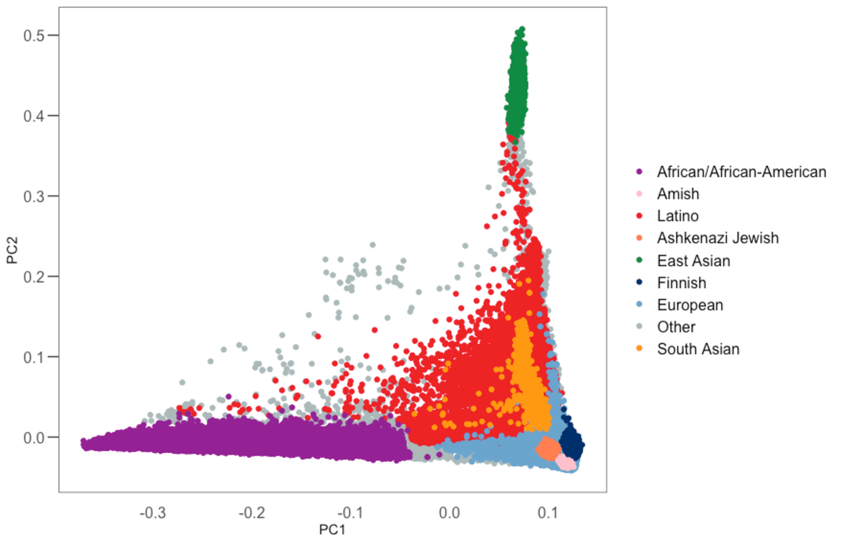
Ancestry assignment
We use principal components analysis (PCA,
hwe_normalized_pc function in Hail)
on our set of high quality variants to compute the first 10 PCs in our samples, excluding first and
second degree relatives. We then train a random forest classifier using 17,906 samples with known
ancestry, and 14,949 samples for which we had a population label from gnomAD v2, as training
samples and using the PCs as features. We assigned ancestry to all samples for which the
probability of that ancestry is > 90% according to the random forest model. All other samples were
assigned the other ancestry (oth).
QC metrics filtering
For this release, we took a different strategy in order to filter outlier samples based on QC metrics: instead of grouping the samples based on their ancestry assignments, we instead regressed out the PCs computed during the ancestry assignment and filtered samples based on the residuals for each of the QC metrics. This strategy allowed us to consider the samples’ ancestry as a continuous spectrum and was particularly beneficial for admixed samples and samples that did not get an ancestry assignment (previously, we lumped all these samples together even though they were drawn from multiple populations).
To illustrate the improvement from this new method, here is the n_snp metric distribution for the
African ancestry samples using our previous and current approaches
| Previous approach | New approach |
|---|---|
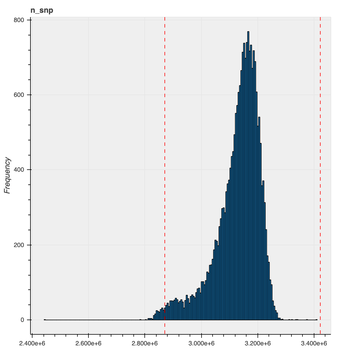 |
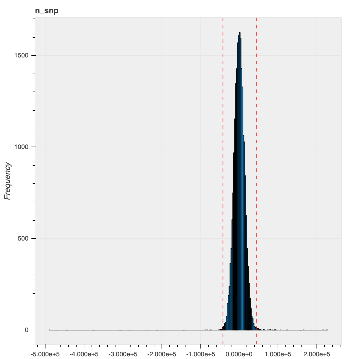 |
We used the sample QC metrics computed using the
Hail sample_qc
module on all autosomal bi-allelic SNVs and filtered samples that were 4 median absolute deviations
(MADs) from the median for the following metrics: n_snp, r_ti_tv,r_insertion_deletion,
n_insertion, n_deletion, r_het_hom_var, n_het, n_hom_var, n_transition and
n_transversion. In addition, we also filtered out samples that were in excess of 8 MADs from the
median number of singletons (n_singleton metric).
Variant QC
For this release, we computed all our variant QC metrics within Hail and because our new sparse format contains all the GVCFs information, we computed them for each allele separately. We then used the allele-specific version of GATK Variant Quality Score Recalibration (VQSR) to compute a confidence score for each allele in our data to be real or artifactual. We used the following features:
- SNPs:
FS,SOR,ReadPosRankSum,MQRankSum,QD,DP,MQ - indels:
FS,SOR,ReadPosRankSum,MQRankSum,QD,DP
On top of the GATK bundle training resources (hapmap, omni, 1000 genomes, mills indels), we also used 10M transmitted singletons (alleles observed exactly twice confidently in a parent and a child) from 6,044 trios present in our raw data.
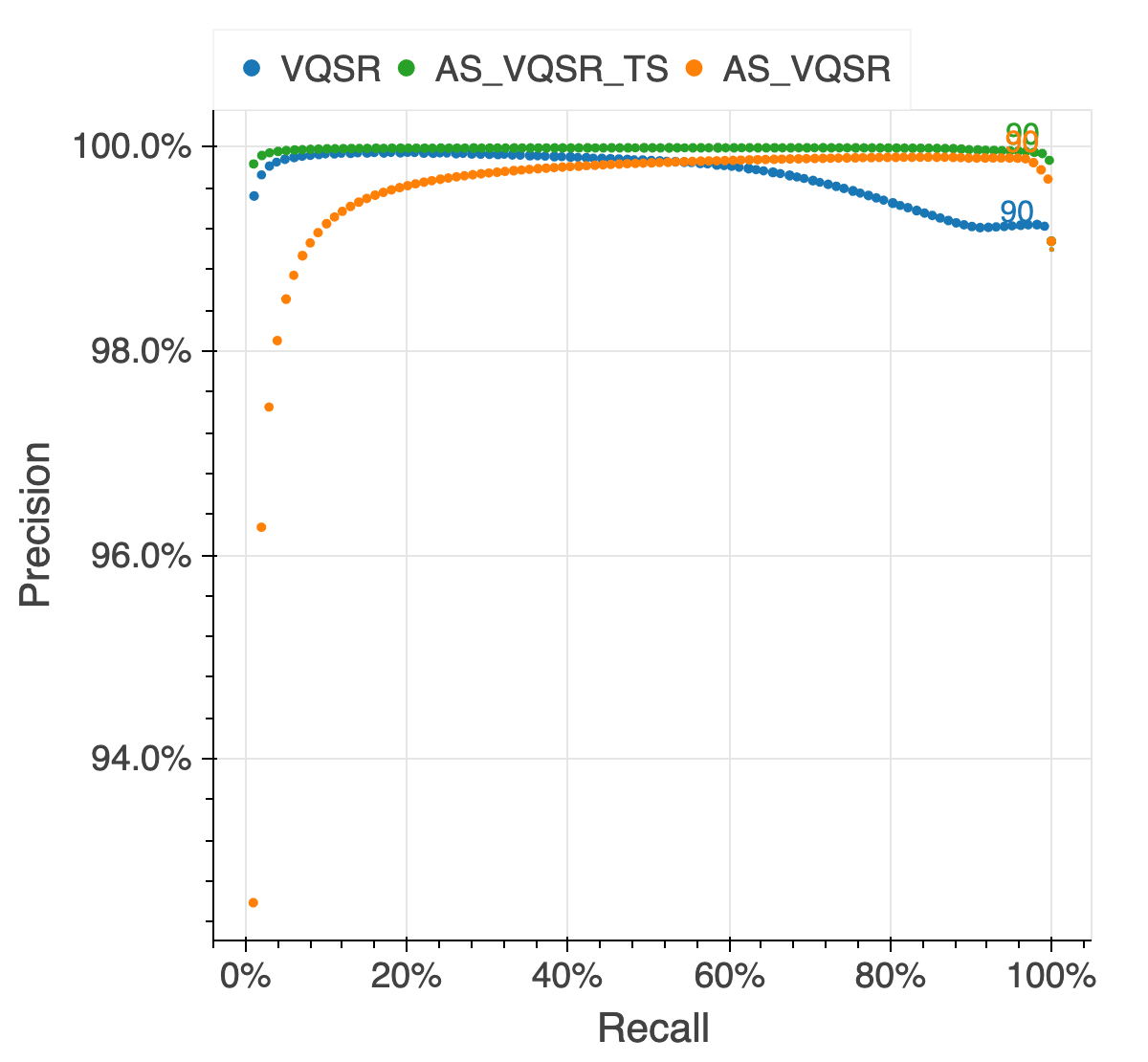
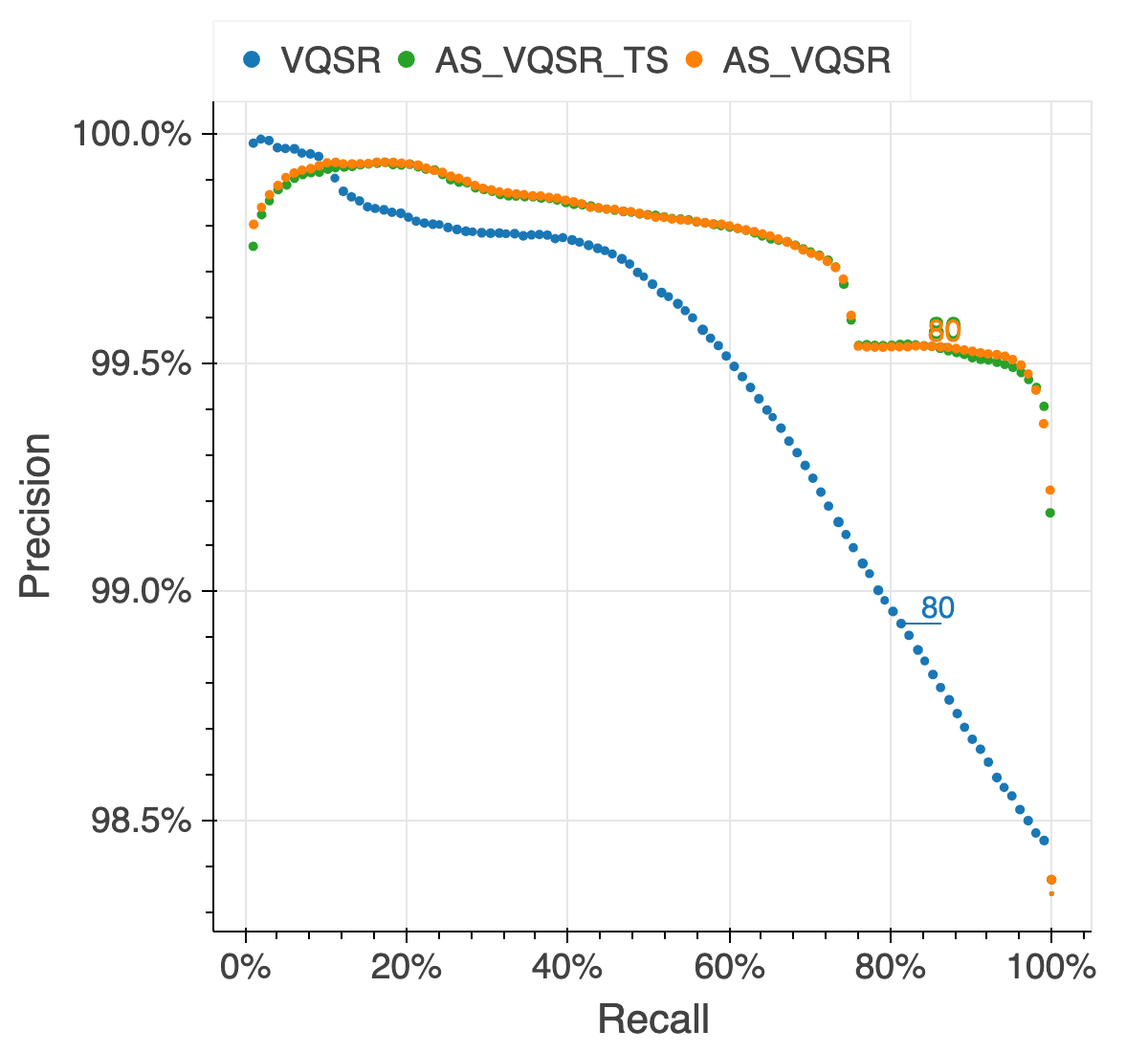
We assessed the results of the filtering by looking at the same quality metrics we used for the gnomAD v2 callset: de novo looking mutations in our 6,044 trios, Ti/Tv ratio, proportion singletons, proportion bi-allelic variants, variants in ClinVar and precision and recall in two truth samples present in our data: NA12878 and a pseudo-diploid sample (A mixture of DNA (est. 50.7% / 49.3%) from two haploid CHM cell lines) for which we have good truth data.
The figure below illustrates the performance of the approach we used (AS_VQSR_TS), compared to
classical site-level VQSR (VQSR) and allele-specific VQSR trained without the transmitted
singletons data (AS_VQSR) on NA12878.
| NA12878 SNVs | NA12878 Indels |
|---|---|
 |
 |
In addition to VQSR, we also applied the following hard filters:
AC0: No sample had a high quality genotype at this variant site (GQ>=20, DP>=10 and allele balance > 0.2 for heterozygotes)InbreedingCoeff: there was an excess of heterozygotes at the site compared to Hardy-Weinberg expectations using a threshold of -0.3 on theInbreedingCoefficientmetric.
In total, 12.7% of SNVs and 34.2% of indels were filtered, leaving 526,001,545 SNVs and 69,168,024 indels that passed all filters in our release.