Originally published on the MacArthur Lab blog.

The first gnomAD structural variant (SV) callset is now available via the gnomAD website and integrated directly into the gnomAD Browser.

This initial gnomAD SV callset includes nearly a half-million distinct SVs across seven SV mutational classes and 13 subclasses of complex SVs detected in 14,891 genomes spanning four major global populations. In the publicly released callset and gnomAD browser, you can find site, frequency, and annotation data for ~445k SVs from 10,738 unrelated genomes with appropriate consent to allow the release of this information.
In this post we summarize how we created this new call set, and some important practical considerations when using it. You can get more details, including callset generation and analyses, in the full gnomad-SV preprint available on bioRxiv.

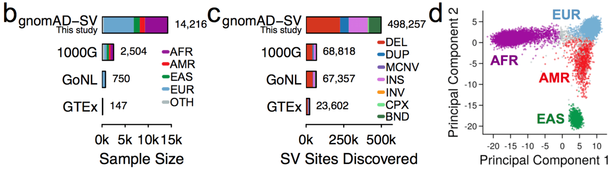
We jointly analyzed 14,891 genomes, 14,216 (95.5%) of which passed initial data quality thresholds, using a multi-algorithm consensus approach (details below) to construct the initial gnomAD SV callset. These samples were all sequenced with 150bp Illumina reads to an average coverage of 32X, and were aligned to the GRCh37/hg19 reference genome. Like previous gnomAD releases, this cohort was aggregated across various population genetic and complex disease studies, and most (57.4%) of the gnomAD-SV cohort overlaps with the genomes included in the current (v2.1) gnomAD SNV and indel allset (for more details, see the supplementary information for the gnomAD-SV preprint.

We subdivided samples into four continental populations and one “other” category, as follows:

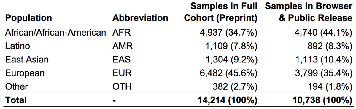
In the gnomAD Browser and the released VCF, we provide variant frequencies separately for each of the four major populations as well as the “other” category.

As with the SNV & indel callset, the subset of 10,738 genomes represented in the gnomAD browser have been screened to remove first-degree relatives and samples with documented pediatric or severe disease. Thus, the publicly available SV data from these 10,738 genomes represents a relatively diverse collection of unrelated individuals that should have rates of most severe diseases equivalent to, if not lower than, the general population.

The gnomAD SV callset

In gnomAD, our working definition of SVs includes all genomic rearrangements involving at least 50bp of DNA, which can be categorized into mutational classes based on their breakpoint signature(s) and/or changes in copy number.

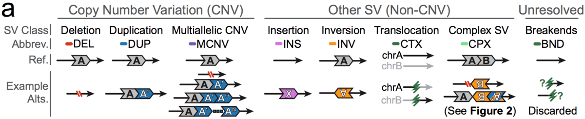
The mutational classes of SVs can be subdivided into two groups:

• Unbalanced SVs are rearrangements that result in gains or losses of genomic DNA (also known as copy number variants, or CNVs)
• Balanced SVs are rearrangements that do not involve changes in copy number

Additionally, each SV can be described as canonical or complex:

• Canonical SVs are rearrangements that involve a single distinct breakpoint signature and/or changes in copy number
• Complex SVs are rearrangements that involve two or more distinct breakpoint signatures and/or changes in copy number

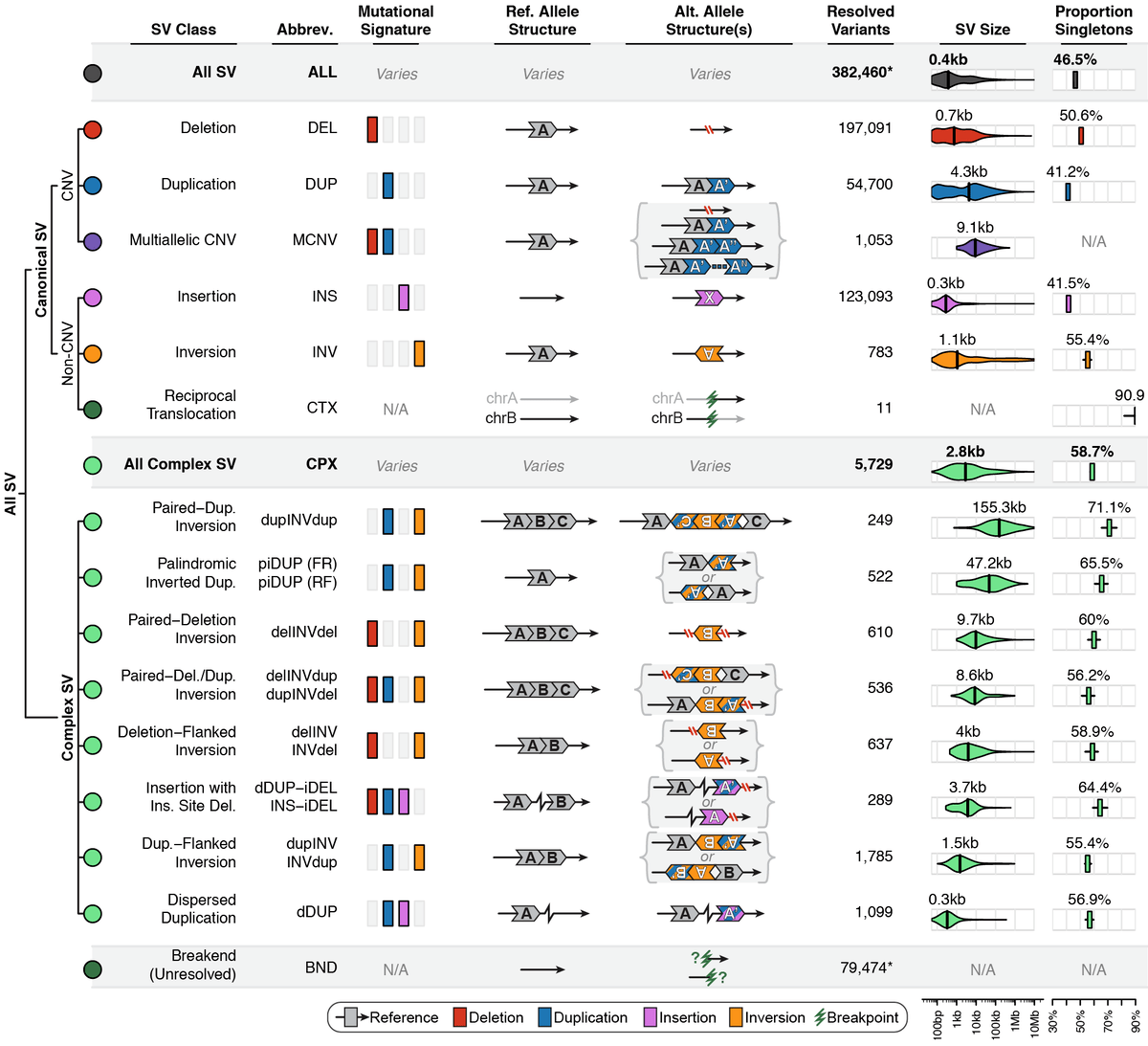
Across the full gnomAD-SV dataset, we discovered a total of 498,257 distinct SVs appearing in one or more genomes, 382,460 of which (76.8%) were completely resolved and appeared in a subset of 12,549 unrelated genomes used in the formal analyses presented in the gnomAD SV preprint. We categorized SVs into the following mutational classes (note: numbers correspond to the final set of SVs from 12,549 unrelated genomes used in the gnomAD SV preprint):

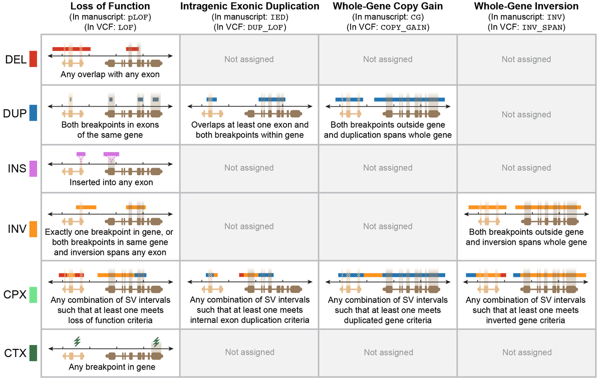
A main aim of producing this gnomAD-SV callset was to supplement existing resources by characterizing which genes in the genome are known to tolerate alteration by SVs, and specifically which kinds of rearrangement these genes can tolerate.

We annotated each SV for multiple potential genic effects using an approach described in the gnomAD SV preprint. In brief, this approach considers SV size, class, position, and overlap with exons from canonical transcripts of Gencode v19 protein-coding genes, which can be graphically summarized below for four main categories SV-gene interactions:

SVs in the gnomAD Browser

One of the most noteworthy aspects of the gnomAD-SV release is the direct integration of SVs into the gnomAD Browser, an effort led by the talented duo of developers, Nick Watts and Matt Solomonson.

In the near future. we intend to produce a short tutorial video covering these features. For now, you can start using the SV features right away with these two easy steps:

1. Navigate to your favorite gene or region using the search bar:

2. Select the SV dataset by clicking the toggle button in the top-right part of the screen:

Once you’ve activated SV mode in the gnomAD Browser, you can interact with the data in multiple ways, described below.

The variant track displays all SVs currently in the view range corresponding to their coordinates, with each SV on its own row.

In the variant track, certain symbols are assigned to specific classes of SV, such as a triangle for insertions (denoting the position at which sequence was inserted), or a lightning bolt for breakpoints of chromosomal translocations or unresolved breakends.

The variant table provides selected metadata for each variant displayed in the variant track, including allele frequencies, consequences, number of homozygotes, coordinates, and size.

All columns in the table are sortable by clicking the column headers.

There are three main options for filtering the variant track & table:

1. Filter by consequence by selecting any combination of consequences in the top row of checkboxes below the variant track
2. Filter by SV class by clicking any combination of buttons in the bottom row below the variant track
3. Filter by keyword by entering that keyword into the search field

For more details about each of these filters, there are help text pop-ups available by clicking the ”?” next to each row of filter buttons.

We provide two options for coloring the SV data: color-by-consequence and color-by-class. You can toggle between these modes using the button directly above the variant track on the right side of the page. The current color key will be reflected by the colors used for the two sets of filter buttons found directly below the variant track.

By default, low-quality variants–such as unresolved breakends–will not be displayed in the variant track or table. You can activate these variants using the checkbox labeled “Include filtered variants” directly above the variant table.

Both the variant track and table are synchronized: any filter, sort, scroll, or highlight applied to one will synchronously be applied to the other. For example, hovering over a single row in the variant table will draw a dashed box to highlighting that SV in the table, but will also highlight that same variant and its position in the track (and vice versa).

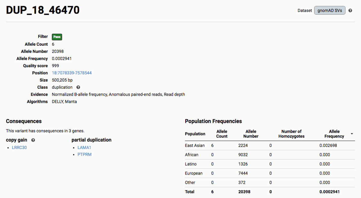
To find more information about an individual variant, you can click on the variant ID in the table or on the variant itself in the track to access the variant page. This page features additional details on the variant, including which algorithms and evidence types contributed to its discovery, its allele frequencies across continental populations, and a full list of all predicted genic consequences.

If you’re ever unsure about what a given SV represents or what its functional consequences mean, visit that variant’s page and click on any of the ”?” help buttons for more information. This is particularly useful for complex SVs, where each help popup gives a graphical representation of the alternate allele structure.

Multiallelic CNVs, which are sites in the genome that have a variable range of copy numbers across individuals in the population, have an extra feature for their variant pages: the distribution of copy numbers in the gnomAD-SV cohort. While we do not phase these regions and/or resolve their individual underlying copy number haplotypes, we provide an aggregate copy number for that locus in sum across both chromosomes per individual. This is represented as a histogram, which has a mouse-over tooltip to show how many individuals are present at each copy state.

Practical considerations when using the gnomAD-SV callset

Below, we list a few important rules-of-thumb to keep in mind when using the gnomAD-SV callset:

• Breakpoint resolution is variable: the resolution of breakpoints varies by the type(s) of evidence contributing to the call, which are marked in the INFO field of the VCF and displayed in the gnomAD browser. Broadly, this means:
  • Variants with split read evidence are accurate within ~tens of bases
  • Variants with discordant read-pair evidence (but no split read evidence) are accurate within ~tens-to-hundreds of bases
  • Variants with read depth evidence (but no split read or read-pair evidence) are accurate within ~hundreds of bases
• Other algorithms and technologies may capture variants missed by gnomAD: although short-read WGS is capable of detecting a broad spectrum of SV classes, it has notable limitations compared to long-read WGS and other approaches. Furthermore, while the four algorithms (Manta, DELLY, MELT, and cn.MOPS) capture a significant fraction of SVs accessible to short-read WGS by comparison to most previous studies, they will certainly not capture all SVs (for instance, small (<300bp) duplications are a known limitation of the current gnomAD callset). Primary sequence context is the most important factor to consider when evaluating SVs ascertained by short-read WGS (such as the data used to build gnomAD-SV). For instance, short-read WGS has limited sensitivity todetect SVs in regions of low-complexity and highly repetitive sequence by comparison to technologies like long-read WGS (i.e., PacBio, Nanopore), optical mapping, or linked-read WGS. In practice, we find short-read WGS performs poorest in regions of segmental duplication (also known as low-copy repeats) or simple repeats.
• Gene consequence annotations are predictions: please note that the gene consequence annotations we generated for gnomAD-SV are predictions, and may not always hold true on a site-by-site basis. Further, we are unable to subdivide our gene consequence annotations for SVs into “low-confidence” and “high-confidence” subsets, such as is performed by LOFTEE for SNVs and indels. Thus, we request that you please carefully inspect each putatively functional SV before interpretation, particularly in the context of its exonic overlap and affected transcripts.
• Manual review of all variants has not been conducted: given the size of this dataset, it is not feasible to curate each variant call. Thus, it is expected that some SVs included in this release represent false and/or misrepresented variant calls, consistent with the range of error rate estimates reported in the gnomAD-SV preprint (~2-12%; see Supplementary Table 4). If you find a variant that appears to meet these criteria, please report the variant.

gnomAD SV discovery methods

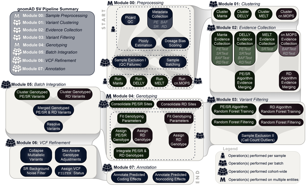
To discover and genotype SVs in this cohort, we extended a multi-algorithm consensus framework from a previous study. You can find technical details on this approach in the methods of Werling et al. (2018) and in the gnomad-SV preprint.

In this new iteration of the SV pipeline, now dubbed the gnomAD SV Discovery Pipeline, we have configured all methods to be executed on Google Cloud via the Workflow Description Language (WDL) and the Cromwell Execution Engine. For gnomAD-SV, these methods were deployed on FireCloud (now known as Terra), a user-friendly interface for massively parallel computing and managing large bioinformatics workflows in the cloud.

At a high level, the general approach taken by the gnomAD SV Discovery Pipeline can be summarized by the following five steps:

• Executes four independent SV detection algorithms (Manta, DELLY, MELT, and cn.MOPS) per sample
• Integrates raw outputs across algorithms and samples
• Filters calls based on four classes of direct evidence available from raw WGS data (anomalous paired-end reads, read depth, split reads, and B-allele SNP frequencies)
• Genotypes all candidate breakpoints across all samples
• Resolves complex SVs, compound heterozygous sites, multiallelic CNVs, performs sex-aware allosome genotype adjustment, and many more steps to refine variant calls

We have provided all components of this pipeline as WDLs, which are available via the FireCloud Methods Repository. Additional details on code availability can be found in the gnomAD-SV supplement.

For the SV callset described in the gnomAD-SV preprint and the callset released via the gnomAD Browser, we performed extensive QC, applied a series of additional filters, and conducted multiple benchmarking analyses. You can read more about the process of producing the gnomAD-SV callset in the supplement of the gnomAD-SV preprint.

Acknowledgements

The creation of gnomAD-SV would not have been possible without the PIs, researchers, and participants of each study that contributed data towards this overall aggregation effort. We would also like to thank the members of the Talkowski Laboratory, the MacArthur Laboratory, the Analytical and Translational Genetics Unit (ATGU) at MGH, and the Broad-SV Group, all of whom provided valuable insight and feedback throughout the process. Specifically, we are grateful to Nick Watts and Matt Solomonson, who developed the new SV features for the gnomAD Browser. Additional acknowledgements, including grants and grant numbers, are listed in the gnomAD-SV preprint.