Originally published on the MacArthur Lab blog.
We are delighted to announce the release of gnomAD v2.1! This new release of gnomAD is based on the same underlying callset as gnomAD v2.0.2, but has the following improvements and new features:
- An awesome new browser
- Per-gene loss-of-function constraint
- Improved sample and variant filtering processes
- Allele frequencies in sub-continental populations in Europe and East Asia
- Allele frequencies computed for the following subsets of the data:
- Controls-only (no cases from common disease case/control studies)
- Samples not assessed for a neurological phenotype
- Samples that were not part of a cancer cohort
- Samples that are not part of the Trans-Omics for Precision Medicine (TOPMed)-BRAVO dataset
- New annotations for each variant
- Filtering allele frequency using Poisson 95% and 99% CI, per population
- Age histogram of heterozygous and homozygous carriers
gnomAD v2.1 comprises a total of 16mln SNVs and 1.2mln indels from 125,748 exomes, and 229mln SNVs and 33mln indels from 15,708 genomes. In addition to the 7 populations already present in gnomAD 2.0.2, this release now breaks down the non-Finnish Europeans and East Asian populations further into sub-populations. The population breakdown is detailed below.
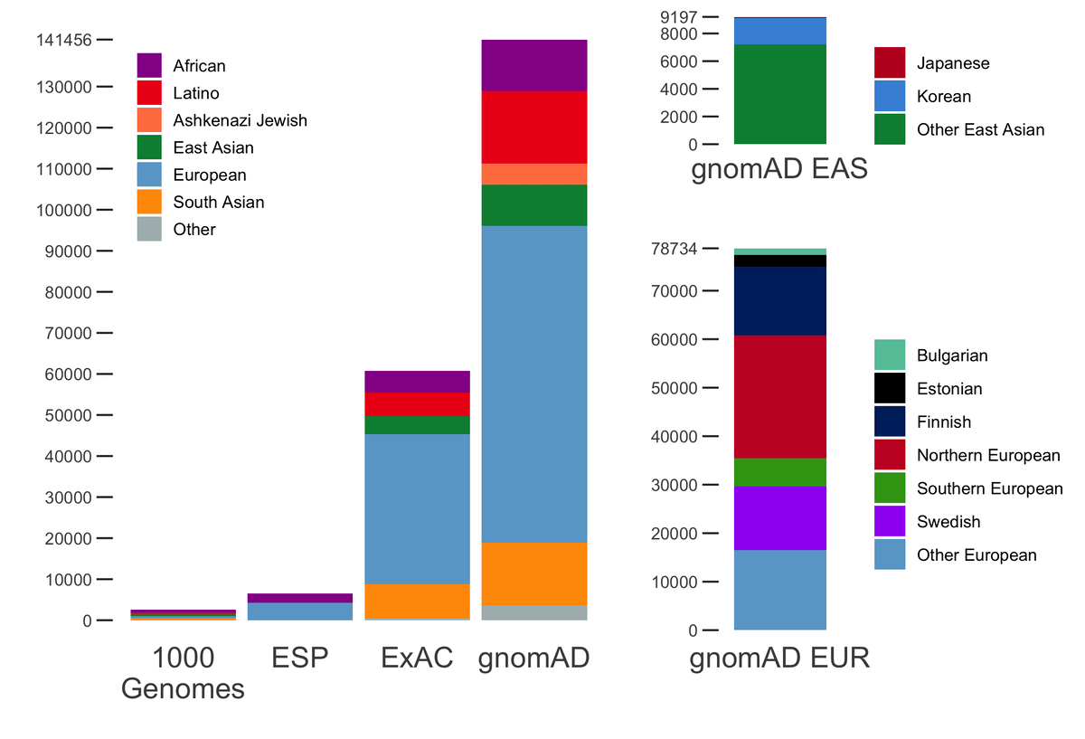
| Population | Description | Genomes | Exomes | Total |
|---|---|---|---|---|
| afr | African/African American | 4,359 | 8,128 | 12,487 |
| amr | Latino/Admixed American | 424 | 17,296 | 17,720 |
| asj | Ashkenazi Jewish | 145 | 5,040 | 5,185 |
| eas | East Asian | (780) | (9,197) | (9,977) |
| kor | Koreans | 0 | 1,909 | 1,909 |
| jpn | Japanese | 0 | 76 | 76 |
| oea | Other East Asian | 780 | 7,212 | 7,992 |
| fin | Finnish | 1,738 | 10,824 | 12,562 |
| nfe | Non-Finnish European | (7,718) | (56,885) | (64,603) |
| bgr | Bulgarian | 0 | 1,335 | 1,335 |
| est | Estonian | 2,297 | 121 | 2,418 |
| nwe | North-Western European | 4,299 | 21,111 | 25,410 |
| seu | Southern European | 53 | 5,752 | 5,805 |
| swe | Swedish | 0 | 13,067 | 13,067 |
| onf | Other non-Finnish European | 1,069 | 15,499 | 16,568 |
| sas | South Asian | 0 | 15,308 | 15,308 |
| oth | Other (population not assigned) | 544 | 3,070 | 3,614 |
| Total | 15,708 | 125,748 | 141,456 |
While the vast majority of these samples were also part of our previous release, our improved sample QC pipeline resulted in a few changes summarized in the table below:
| Overlapping | In 2.0.2 only | In 2.1 only | |
|---|---|---|---|
| Genomes | 14,977 | 519 | 731 |
| Exomes | 119,116 | 4,020 | 6,632 |
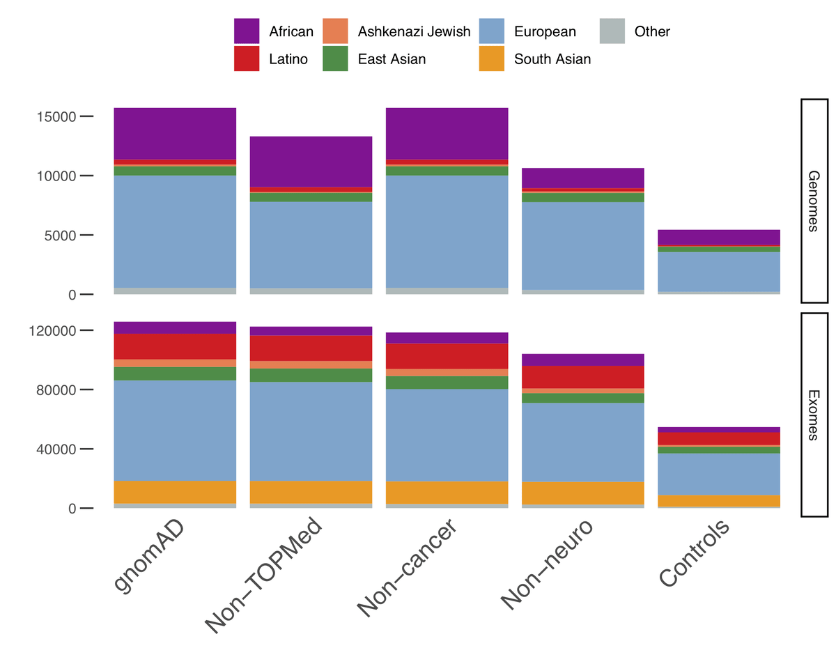
In addition to providing allele-frequencies for sub-continental populations, we have also computed allele-frequencies on subsets of the data of particular interest:
- Non-TOPMed: only samples that are not present in the Trans-Omics for Precision Medicine (TOPMed)- BRAVO release. The allele counts in this subset can thus be added to those of BRAVO to federate both datasets.
- Non-cancer: Only samples from individuals who were not ascertained for having cancer in a cancer study
- Non-neuro: Only samples from individuals who were not ascertained for having a neurological condition in a neurological case/control study
- Controls-only: Only samples from individuals who were not selected as a case in a case/control study of common disease
As it has always been, gnomAD is available for download and on our browser and can be used freely by anyone without any restrictions. We are preparing a series of papers that will present some of the exciting scientific insights that can be gleaned from these data.
Changes in the release VCF and Hail Table
New annotations: Filtering allele frequency and age histograms
With gnomAD 2.1, two new annotations are available for each variant:
- Filtering allele frequency: this annotation contains a threshold filter allele frequency for a variant. If the filter allele frequency of a variant is above the maximum credible populationAF for a condition of interest, then that variant should not be considered a plausible candidate ausative variant (see http://cardiodb.org/allelefrequencyapp/). This annotation is computed globally and for each population separately. Two thresholds are available for each population: 95% CI and 99% CI.
- Age histograms: For each variant, histogram of the age of heterozygous and homozygous carriers
are available. The format for those is a pipe-delimited string of counts from age 30 to 80 by
increments of 5 years. Counts of individuals below and above these thresholds are available in
the
age_hist_*_n_smallerandage_hist_*_n_largerfields (where * can behetorhom).
Split all the multi-allelic variants
For this release, all multi-allelic sites have been split. This means that multiple lines now have the same chromosome and position. This decision was made since the vast majority (all?) of gnomAD downstream users did not want to have multiple alleles on a single line.
Hemizygote counts
For this release, there are no more hemizygote count annotations. Instead, our male counts
correctly consider males as hemizygous in non-pseudo-autosomal (non-PAR) regions of the sex
chromosomes and we provide a nonpar flag to identify all variants that are in the these regions.
Flagging, but not filtering problematic regions
We have moved the information about sites falling in low complexity (lcr), decoy (decoy) and
segmental duplication (segdup) regions to the INFO field. This means that the information is
still easily available in the VCF and Hail Table, but variants in these regions that pass other
filters will have a PASS value in the FILTER column. In the browser, lcr, decoy and
segdup are displayed in the Flags column.
The end of SHOUTING population names
It has been a tradition in the VCF annotations to SHOUT things. With this release, we have decided
that while we would keep all original VCF and GATK annotations with their letter case (e.g. AC,
AN, AF), gnomAD populations, subsets, etc. will be lowercase. As an example, the allele
frequency for African male samples is stored in AF_afr_male.
Hail Table gets a new schema
For those using Hail to perform their analyses (highly recommended!), this new release comes with a different schema than gnomAD v.2.0.2. Instead of having a nested schema for the different subsets/populations/sex, all similar annotations are stored in an array. There are 5 such arrays at the root of the row schema:
freq: Allele frequency information (AC, AN, AF, homozygote count)age_hist_het: Histogram of heterozygous carriersage_hist_hom: Histogram of homozygous carrierspopmax: Allele frequency information for the non-bottlenecked population with the highest frequency. This excludes Ashkenazi Jewish (asj), European Finnish (fin), and “Other” (oth) populations.faf: Filtering allele frequency (see definition above)
For each variant, these arrays contain the subsets/populations/sex combinations in a predetermined order. To find the correct index for a given combination of subset/population/sex, we provide a global index for each array:
freq_index_dictforfreqage_index_dictforage_hist_hetandage_hist_hompopmax_index_dictforpopmaxfaf_index_dictforfaf
This structure allows users to prepare a desired expression by looking into the index (often programatically) and then accessing the desired element(s) in the array(s) through an expression.
Constraint
With this release, we are finally releasing new per-gene constraint scores computed with gnomAD! These scores can either be downloaded as a table or viewed on the gnomAD browser.
With gnomAD, we have shifted from using the probability of being loss-of-function intolerant (pLI) score developed with ExAC and now recommend using the observed / expected score. For this reason, the constraint table displayed on the browser (unless the ExAC data is selected) now also shows the observed / expected (oe) metric. It is very important to note that the scale of oe is very different from that of pLI; in particular low oe values are indicative of strong intolerance. In addition, while pLI incorporated the uncertainty around low counts (i.e a gene with low expected count could not have a high pLI), oe does not. Therefore, the oe metric comes with a 90% CI. It is important to consider the confidence interval when using oe.
The change from pLI to oe was motivated mainly by its easier interpretation and its continuity across the spectrum of selection. As an example, let’s take a gene with a pLI of 0.8: this means that this gene cannot be categorized as a highly likely haploinsufficient gene based on our data. However, it is unclear whether this value was obtained because of sample size or because there were too many loss-of-function (LoF) variants observed in the gene. In addition, if the cause was the latter, pLI doesn’t tell much about the overall selection against loss-of-function in this gene. On the other hand, a gene with a LoF oe of 0.4 can clearly be interpreted as a gene where only 40% of the expected loss-of-function variants were observed and therefore is likely under selection against LoF variants. In addition, the oe 90% CI allows us to clearly distinguish cases where there is a lot of uncertainty about the constraint for that gene due to sample size.
Since pLI > 0.9 is widely used in research and clinical interpretation of Mendelian cases, we suggest using the upper bound of the oe confidence interval < 0.35 if a hard threshold is needed. Note that we also provide pLI values computed with gnomAD.
The new gnomAD browser
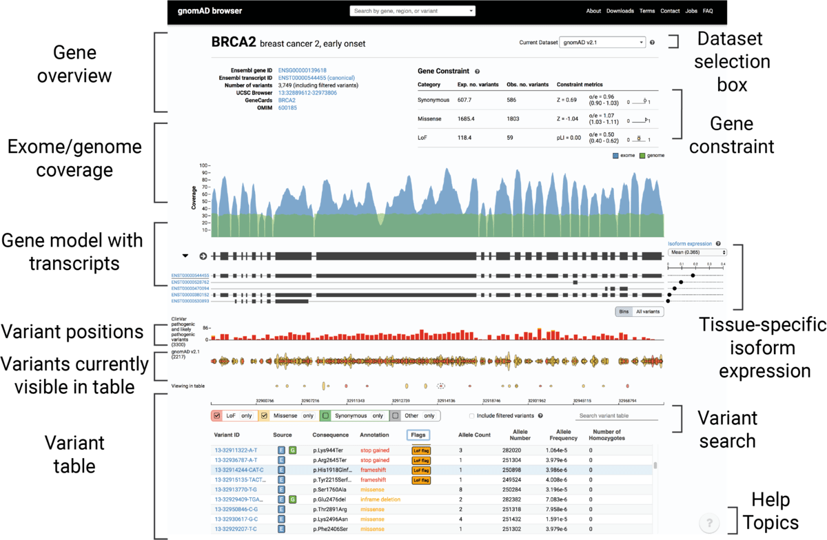
We are very excited to announce the release of the newly redesigned and re-engineered gnomAD browser! We kept aesthetic and utility of the original ExAC/gnomAD browsers while bringing the following improvements:
- Improved browsing performance/loading times; all genes should load successfully. If you find a gene that does not load, please email us
- Support for viewing subsets and ExAC
- Multiple new features on our gene and variants pages, including
- Gene page
- Gene model with multiple transcripts along with isoform expression from GTex
- Regional missense constraint (available for ExAC dataset only)
- ClinVar variants track
- Entirely redesigned variants table
- Variants page
- Filtering allele frequency annotations
- Sub-continental population breakdown
- Age histograms for heterozygote and homozygote carriers
- Gene page
- A brand new region view: Specific intervals of the genome can be viewed using with a query
formatted as
chrom-start-stop. We’ve capped the number of variants returnable for this search at 30,000. If your query is larger than this, the coverage and genes will still return but you’ll be asked to make your interval smaller. You can also click on a gene in the region to be taken to the gene page for that gene. (For example, try region: 1-55405222-55630526) - Intuitive help system
- Behind-the-scenes technology improvements that improve user experience and allow us to develop new features more quickly
- Database and infrastructure improvements that address the increasing size and complexity of gnomAD
Sample QC
The overall sample QC process is similar to the 2.0.2 pipeline. The most profound difference is a much refined sequencing platform assignment process, especially for the exomes for which we developed a data-driven platform assignment method (step 2 bellow). In addition, we have now implemented the entire pipeline using Hail, requiring no external software (except for Picard tools for the sequencing quality metrics). The process followed the following steps:
- Exclude samples based on hard thresholds on sequencing and raw calls metrics
- Assign sequencing platform
- Exclude relatives (up to 2nd degree relatives)
- Infer ancestry using PCA
- Exclude samples that are outliers for calling quality metrics in their ancestry/platform group.
Steps 1 and 2 were performed on exomes and genomes separately, whereas the rest of the pipeline was performed on the combined data. These steps are described in more details in the next sections.
1. Hard filtering
The hard filtering process was very similar to that of gnomAD 2.0.2, with the addition of a raw call rate cutoff at 0.85 and refined sex abnormality filters in exomes. In addition, all calling metrics were computed using Hail. We excluded samples based on the following thresholds:
- Both exomes and genomes:
- High contamination: freemix > 0.05
- Low call rate: callrate < 0.85
- Excess chimeric reads: pct_chimera > 0.05
- Exomes only
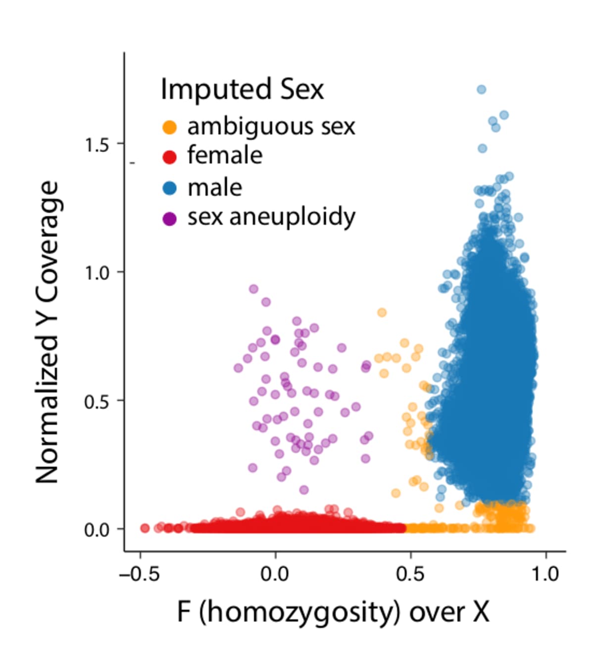
- No coverage: Average chrom20 coverage = 0
- Ambiguous sex (see plot below):
- F inbreeding on X (non-PAR) >= 0.5 & normalized Y chromosome coverage <= 0.1
- 0.6 <= F inbreeding on X (non-PAR) >= 0.4 & normalized Y chromosome coverage > 0.1
- Sex aneuploidies
- F inbreeding on X (non-PAR) < 0.4 & normalized Y chromosome coverage > 0.1
- Genomes only
- Low coverage: mean coverage < 15x
- Small insert size: Median insert size < 250bp
- Ambiguous sex: fell outside of:
- Male: chromosome X F-stat > 0.8
- Female: chromosome X F-stat < 0.4
2. Assign sequencing platform
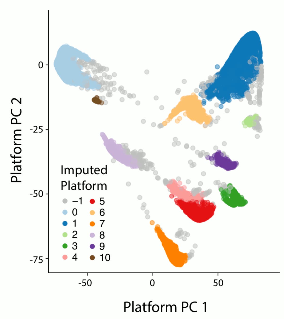
The platform on which a sample is sequenced is a crucial determinant of the genomic information captured in that sample. Because our pipeline relies on an outlier detection strategy, it is very important that we apply that process to samples that were sequenced using a similar technology. For this new release, we have substantially improved our sequencing platform assignment as described below. This change is the most dramatic change in our sample QC process.
Genomes
Since all the genomes in gnomAD v2 were sequenced at the Broad Institute, we have complete and detailed metadata for these samples. For this release, instead of classifying the genomes solely based on whether they used a PCR+ or PCR-free preparation process, we used the exact version of the protocol used for each sample. In total, we divided our genomes in 9 different sequencing protocols.
Exomes
One of the major refinements to our sample QC pipeline is the introduction of a data-driven method to automatically discover and assign exome platforms. In our previous release, we had relied on metadata from the different projects that compose gnomAD to assign exome samples to a sequencing platform. This approach had two major caveats: first, many samples lacked this information and were thus lumped in an “other platform” category that was difficult to use for filtering as it grouped a collection of very different sequencing platforms that had different capture targets and coverage profiles. Second, the annotations provided were sometimes inaccurate, for example in the case of project that used different capture kits over time. Our method differentiates the different exome sequencing capture kits based on their capture targets. For each capture target in our well-behaved calling regions (as defined by GATK), we assigned a binary annotation to each sample based on whether this sample had a call rate above or below 25%. We then computed the 9 first principal components (PCs) of the resulting target-by-sample matrix using the pca method in Hail. Finally we used hierarchical density-based spatial clustering of applications with noise (HDBSCAN from the sklearn python package) to cluster our samples based on their PC values. When compared to labels from project where we knew the major exome sequencing platform, 97.7% of these were correctly assigned to their respective cluster (96.7% for agilent, 99% for ICE, 96.9% for ICE with 150bp read length and 100% for nimblegen).
3. Relatedness filtering
Relatedness filtering for this release was done very similarly to the 2.0.2 release. The only difference is that instead of using KING, we used the pc_relate method in Hail to infer relatedness. Relatedness was computed amongst all samples that passed the hard filters in both exomes and genomes together. The sites we used for inferring relatedness were defined as follows:
- Present in both exomes and genomes
- Autosomal, bi-allelic single nucleotide variants (SNVs) only
- Allele frequency > 0.1%
- Call rate > 99%
- LD-pruned with a cutoff of r2 = 0.1
After running pc_relate, we used the maximal_independent_set method in Hail to get the largest set of samples with no pair of samples related at the 2nd degree or closer. When we had to select a sample amongst multiple possibilities, we used the same scheme to favor a sample over another:
- Genomes had priority over exomes
- Within genomes
- PCR free had priority over PCR+
- In a parent/child pair, the parent was kept
- Ties broken by the sample with highest mean coverage
- Within exomes
- Exomes sequenced at the Broad Institute had priority over others
- More recently sequenced samples were given priority (when information available)
- In a parent/child pair, the parent was kept
- Ties broken by the sample with the higher percent bases above 20x
4. Ancestry assignment
The global ancestry assignment was entirely run within the Hail framework but otherwise was the done in the same manner as for release 2.0.2. In addition, we performed sub-continental ancestry assignment Europeans and East Asians. We used principal components analysis (PCA) to assign both global and sub-continental ancestries. The figure below shows a 2D uniform manifold approximation and projection (UMAP) of the global PCs 1-6 and 8, colored by the inferred ancestries of the samples. As can be seen, the different ancestries separate well in PC-space and recapitulate expected geographical proximity between populations.

The process for ancestry assignment is detailed in the next subsections.
Global ancestry assignment
Using the hwe_normalized_pca function in Hail,
we computed the 10 first principal components (PCs) on the same 94,176 well-behaved bi-allelic
autosomal SNVs as described above on all unrelated samples (exomes and genomes combined). We then
leveraged a set of 52,768 samples for which we knew the ancestry to train a random forests
classifier using the PCs as features. We assigned ancestry to all samples for which the probability
of that ancestry was > 90% according to the random forest model. All other samples were assigned
the other ancestry (oth). In addition, the 34 South Asian (sas) samples among the genomes were
assigned to other as well due to their low number.
Sub-continental ancestry assignment
Sub-continental ancestry was computed for European and East Asian samples using PCA. The reason for computing for these two global ancestry groups only was (1) the presence of reliable labels of known sub-population for large enough samples of the data, and (2) the resulting PCA was convincingly splitting the data into separate clusters that matched our known labels. The following steps were taken for the non-Finnish European and East Asian samples separately:
- High-quality sites (same used for relatedness) were extracted for all samples of that global ancestry.
- Sites were further filtered to exclude
- Sites where the allele frequency in that global population was < 0.1%
- Sites where any platform had > 0.1% missingness (or more than 1 missing sample if there were less than 1,000 samples for a given platform)
- Remaining sites were LD-pruned in that population down to r2 = 0.1
- PCs were computed using hwe_normalized_pca in Hail.
- A random forest (RF) model was created using:
- European samples: 3 first PCs as features and known sub-continental population labels for 17,102 samples
- East Asian samples: first 2 PCs as features and known sub-continental population labels for 2,067 samples.
- All samples with a random forest prediction probability > 90% according to the random forest
were assigned a sub-continental populations. Other samples were assigned the other non-Finnish
European (
onf) or other East Asian (oea) ancestry depending on their global ancestry.
5. Stratified QC filtering
Similar to our 2.0.2 release, our final sample QC step was to exclude any sample falling outside 4 median absolute deviations (MAD) from the median of any of the given metrics:
- Number of deletions
- Number of insertions
- Number of SNVs
- Insertion : deletion ratio
- Transition : transversion (TiTv) ratio
- Heterozygous : homozygous ratio
- Call rate (genomes only)
Because these metrics are sensitive to population and sequencing platform, the distributions were computed separately for each global population / platform group. The populations and platforms used are those described above.
Variant QC
For variants QC, we used all sites present in the 141,456 release samples as well as sites present in family members forming trios (212 trios in genomes, 4,568 trios in exomes) that passed all of the sample QC filters. Including these trios allowed us to look at transmission and Mendelian violations for evaluation purposes. Variant QC was performed on the exomes and genomes separately but using the same pipeline (although different thresholds were used).
For the gnomAD release 2.1, we used an improved random forests (RF) model using newly developed annotations. This updated model is described below and performs markedly better than both VQSR and our previous model on all the evaluation metrics we used. In addition to our RF filter, we also excluded all sites failing the following two hard filters:
InbreedingCoeff: Excess heterozygotes defined by an inbreeding coefficient < -0.3AC0: No sample had a high quality genotype (depth >= 10, genotype quality >= 20 and minor allele balance > 0.2 for heterozygous genotypes)
Finally, for this release we have moved the information about sites falling in low complexity
(lcr), decoy (decoy) and segmental duplication (segdup) regions to the INFO field. This
means that the information is still easily available in the VCF but variants in these regions that
pass other filters will have a PASS value in the FILTER column. In the browser, lcr, decoy
and segdup are displayed in the Flags column.
Random forests model
For our previous release, we had introduced a new variant filtering method based on a random forests model, which performed per-allele rather than per-site filtering. For this release, we have kept the model similar but have improved the features it is using for classification. The problem with the features used in 2.0.2 is that they relied heavily on the median sample quality to determine the filtering status of each allele. While this works very well with many samples, median can be unstable when dealing with low number of samples. As an example, if there are only two samples, median values could be really biased if the quality of those samples differ. Because gnomAD aggregates many cohorts sequenced on different platforms, this was sometimes problematic and filtered sites that had good evidence in some samples, but where the median sample was below the model’s quality threshold. For this reason, we dropped the median values entirely and introduced two new metrics:
qd: This metric is inspired by the GATK quality / depth (QD) metric, but is computed per-allele, only on the carriers of that allele. So for each allele,qdis computed as the sum of the non-reference genotype likelihoods divided by the sum of the depth in all carrier of that allele.pab_max: This metric is the highest p-value for sampling the observed allele balance under a binomial model. Because we take the highest value, we effectively consider the “best looking” sample in terms of allele-balance.
Other than that, most of our model building and evaluation was similar to what we used for release 2.0.2.
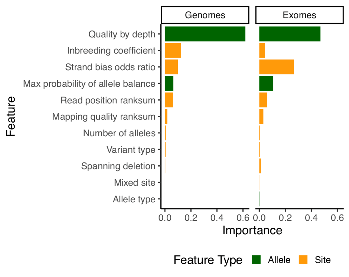
Note that since random forests doesn’t tolerate missing data, we have naively imputed all missing values using the median value for that feature.
Random forest training examples
Our strategy for selecting training sites was the same as for gnomAD v2.0.2; however, because we had an increase in our number of trios, we had more positive transmitted singletons alleles than previously. The table below summarizes our training examples.
| Name | Description | Class | Number of alleles in genomes | Number of alleles in exomes |
|---|---|---|---|---|
| omni | SNVs present on the Omni 2.5 genotyping array and found in 1000 genomes (available in the GATK bundle) | TP | 2.3Mln | 95k |
| mills | Indels present in the Mills and Devine data (available in the GATK bundle) | TP | 1.3Mln | 12k |
| 1000 Genomes high-quality sites | Sites discovered in 1000 Genomes with high confidence (available in the GATK bundle) | TP | 29Mln | 560k |
| transmitted_singletons | variants found in two and only two individuals, which were a parent-offspring pair | TP | 116k | 106k |
| fail_hard_filters | variants failing traditional GATK hard filters: QD < 2 | FS > 60 |
Note that for training the model, we used a balanced training set by randomly downsampling the class that had more training examples to match the number of training examples in the other class.
Random forests filtering thresholds
In order to set a threshold for the PASS / RF filter in the release, we have used a slightly
different set of evaluation metrics. The reason being that some of the classical metrics such as
transition/transversion ratio and insertion:deletion ratio are very difficult to interpret in large
callsets. On the other hand, we have additional data and resources that can serve as useful proxy
for callset quality, such as large number of trios, validated variants (e.g. validated de novo
mutations in our exomes) or public databases such as ClinVar. We used the following metrics to
determine a cutoff on the random forests model output, to build what we believed to be a high
quality set of variants:
- Precision / recall against two well characterized samples:
- NA12878 from genome in a bottle
- CHM1_CHM13: A mixture of DNA (est. 50.7% / 49.3%) from two haploid CHM cell lines, deep sequenced with PacBio and de novo assembled, available here. Note that indels of size 1 were removed because of PacBio-specific problems.
- Number of singleton Mendelian violations in our evaluation trios (N=1 amongst all samples and is found in a child)
- Singleton transmission ratio in trios
- Sensitivity to validated de novo mutations (exomes only)
- Sensitivity to singleton ClinVar variants
For exomes, our filtration process removes 12.2% of SNVs (RF probability >= 0.1) and 24.7% of indels (RF probability >= 0.2). For genomes, we filtered 10.7% of SNVs (RF probability >= 0.4) and 22.3% of indels (RF probability >= 0.4).
Acknowledgments
The creation of gnomAD 2.1 was an enormous team effort from a large team and we want here to thank the many people that have contributed behind the scenes.
Massive thanks, as always, to everyone who allowed their data to be used in this project. The gnomAD consortium now includes more than 100 principal investigators, who are listed here. We’re grateful to all of them for allowing their data to be used for this project.
Jessica Alföldi played a critical role in communicating with principal investigators, assembling the sample list and gathering the permissions required to ensure that each and every sample in the project was authorized to be included – a seriously daunting task! Fengmei Zhao contributed to the assembly of the underlying data, and Kristen Laricchia and Monkol Lek played important roles in sample and variant quality control.
Ben Weisburd helped with the gnomAD browser, and generated all of the read visualizations you can see on the variant pages.
An enormous thanks to the entire Hail team for working hand in hand with us in order to produce this resource: Cotton Seed, Jon Bloom, Tim Poterba, Jackie Goldstein, Daniel King, Amanda Wang, Patrick Schultz and Chris Vittal. As mentioned, all of our code for quality control, generation of the data and computation of all of the metrics is now done within Hail.
The pipelines and infrastructure required to align and call variants, and the actual generation of the massive exome and genome call sets, are entirely the work of the heroic men and women of the Broad’s Data Sciences Platform. Many people deserve thanks here, but we wanted to single out Eric Banks, Kathleen Tibbetts, Charlotte Tolonen, Yossi Farjoun, Laura Gauthier, Dave Shiga, Jose Soto, George Grant, Sam Novod, Valentin Ruano-Rubio, and Bradley Taylor.
And finally, special thanks to the Broad Institute Genomics Platform as a whole, who generated 90% of the data used in gnomAD, and also provided critical computing resources required for this work.
Post was updated on April 20, 2022 to update popmax population labels and rephrase “outbred population” as “non-bottlenecked population”.