Originally published on the MacArthur Lab blog.
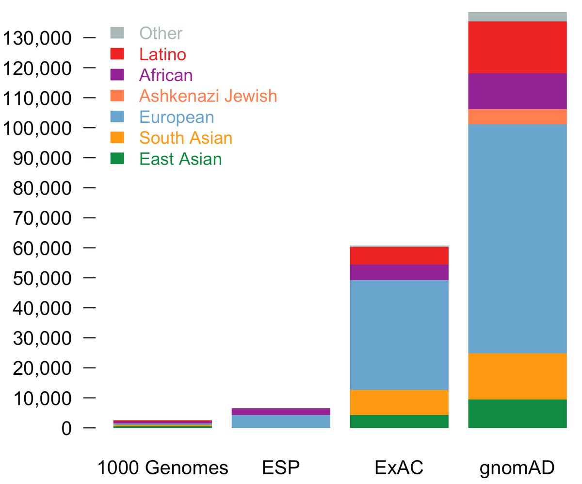
Today, we are pleased to announce the formal release of the genome aggregation database (gnomAD). This release comprises two callsets: exome sequence data from 123,136 individuals and whole genome sequencing from 15,496 individuals. Importantly, in addition to an increased number of individuals of each of the populations in ExAC, we now additionally provide allele frequencies across over 5000 Ashkenazi Jewish (ASJ) individuals.
The population breakdown is detailed in the table below.
| Population | Description | Genomes | Exomes | Total |
|---|---|---|---|---|
| AFR | African/African American | 4,368 | 7,652 | 12,020 |
| AMR | Admixed American | 419 | 16,791 | 17,210 |
| ASJ | Ashkenazi Jewish | 151 | 4,925 | 5,076 |
| EAS | East Asian | 811 | 8,624 | 9,435 |
| FIN | Finnish | 1,747 | 11,150 | 12,897 |
| NFE | Non-Finnish European | 7,509 | 55,860 | 63,369 |
| SAS | South Asian | 0 | 15,391 | 15,391 |
| OTH | Other (population not assigned) | 491 | 2,743 | 3,234 |
| Total | 15,496 | 123,136 | 138,632 |
While the data from gnomAD have been available on the beta gnomAD browser for several months (since our announcement at ASHG last October), this release corresponds to a far more carefully filtered data set that is now available through the gnomAD browser, as well as a sites VCF and a Hail sites VDS for download and analysis at https://gnomad.broadinstitute.org/downloads.
In this blog post, we first describe the major changes from ExAC that will be apparent to users. We then dig into the details of the sample and variant QC done on the gnomAD data. It is important to note that while the alignment and variant calling process was similar to that of ExAC, the sample and variant QC were fairly different. In particular, the vast majority of processing and QC analyses were performed using Hail. This scalable framework was crucial for processing such large datasets in a reasonable amount of time, allowing for exploration of the data at a much more rapid scale. We’d like to extend a special thanks to the Hail team for their support throughout the process, especially Tim Poterba and Cotton Seed.
Important usage notes
These few notes describe important changes from the ExAC dataset.
Changes to the browser
The gnomAD browser is very similar to the ExAC browser with a few modifications to support
integration of genome data. The coverage plot now has a green line to display genome coverage. In
the variant table, a source column indicates whether the variant belongs to the exome callset
(![]() ),
genome callset
(
),
genome callset
(![]() ),
or both callsets
(
),
or both callsets
(![]() and
and ![]() ).
Variants present in both datasets have combined summary statistics (allele count, allele frequency,
etc). We have added checkboxes for specifying which data to display on the page. Users can choose
to include or exclude SNPs, indels, exome variants, genome variants, or filtered (non-pass)
variants and the table statistics update accordingly. If filtered (non-pass) variants are included,
the data source icons will be distinguished with reduced opacity and a dotted border to indicate
lower reliability
(
).
Variants present in both datasets have combined summary statistics (allele count, allele frequency,
etc). We have added checkboxes for specifying which data to display on the page. Users can choose
to include or exclude SNPs, indels, exome variants, genome variants, or filtered (non-pass)
variants and the table statistics update accordingly. If filtered (non-pass) variants are included,
the data source icons will be distinguished with reduced opacity and a dotted border to indicate
lower reliability
(![]() ).
Variants present in both datasets have combined summary statistics (allele count, allele frequency,
etc). A variant’s filter status can be discovered by hovering over the icon (e.g.
).
Variants present in both datasets have combined summary statistics (allele count, allele frequency,
etc). A variant’s filter status can be discovered by hovering over the icon (e.g. AC0, RF). Be
careful when including filtered variants: some poor quality variants (and summary statistics) will
be added to the table. This feature should be used with caution.
On the variant page, the population frequency table has been modified such that exome and genome population statistics can be included or excluded. By default, filtered variants are not included in the population table but can be added by clicking the checkbox.
There is a new “report variant” button on each variant page. Clicking this button opens a submission form where users can express concerns about a variant (such as low quality or clinical implausibility). Users can also request more information about variant carriers. Generally phenotype data is not available for samples in gnomAD as many of the individuals who have contributed data to gnomAD were not fully consented for phenotype data sharing. In the future, it may become available for a small subset of samples with appropriate consents. This is an experimental feature. Due to limited personnel, the gnomAD team may not be able to respond to your submission.
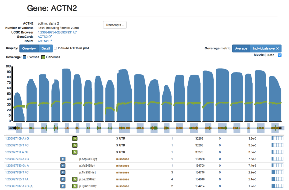
Finally, read data can now be viewed for both exome and genome data (restricted to exome calling intervals only), with up to 3 IGV.js tracks provided for each sample type (heterozygous, homozygous, and hemizygous). If there are more than 3 individuals for one of these sample types, the 3 individuals shown are those that have the highest GQ.
Allele count default is high quality genotypes only
We have changed the default allele count to include only genotypes passing our adjusted threshold
(GQ >= 20, DP >= 10, and have now added: allele balance > 0.2 for heterozygote genotypes),
which was previously in AC_Adj. The raw allele counts are now available in AC_raw. All sites
with no high quality genotype (AC = 0) are marked as filtered using the AC0 filter.
No chromosome Y in genomes
There is no chromosome Y coverage / calls in the gnomAD genomes, because reasons.
Changes in the VCF
By and large, the release VCFs look and feel similar to the ExAC v1 VCF. Exomes and genomes are
distributed separately. We have removed the Het fields as they were hard to parse and instead
provide genotype counts (GC), or a G-indexed array of counts of individuals per genotype. As
mentioned in the Variant QC section, we have fundamentally switched from a site-level filtering
strategy to an allele-specific filtering strategy. For this reason, we now have a field named
AS_FilterStatus in the INFO column that specifies the filtering status for each allele
separately. If any allele is PASS, then the entire site is PASS (unless it is in a LCR or
SEGDUP region, or fails the InbreedingCoeff filter). Finally, we provide VDS format for users
wishing to perform analyses in Hail.
Alignment and variant QC
The alignment and variant calling was performed on exomes and genomes separately using a standardized BWA-Picard pipeline on the human genome build 37, followed by joint variant calling across each whole callset using GATK HaplotypeCaller (v3.4). Up to this point, the pipeline used is very similar to the ExAC pipeline; however, after the variant calling step, there are a number of differences that are worth noting here.
Sample QC process
The sample filtering process was similar to that of ExAC, where we first excluded samples based on sequencing and raw variant call quality metrics, then removed related individuals as to keep only samples more distant than 2nd degree relatives. From this set, we assigned ancestry and finally excluded samples based on raw variant call QC metrics stratified by sequencing platform and ancestry. These steps are detailed below.
Hard filtering
Sequencing and alignment quality metrics were computed using Picard tools and raw quality metrics were computed using GATK, PLINK, and Hail. We have excluded samples based on the following thresholds:
- Both exomes and genomes
- High contamination: freemix > 5%
- Excess chimeric reads: > 5% chimeric reads
- Excess heterozygosity: F < -0.05
- Exomes only
- No coverage: a set of common test SNPs on chromosome 20 had no coverage
- Some TCGA samples (e.g. known tumor) were removed
- Ambiguous sex: fell outside of:
- Male: Proportion of heterozygous sites on chromosome X (non-PAR regions) < 0.2 and chromosome Y coverage > 0.1x
- Female: Proportion of heterozygous sites on chromosome X (non-PAR regions) > 0.2 and chromosome Y coverage < 0.1x
- Genomes only
- Low depth: Mean depth < 15x
- Small insert size: Median insert size < 250bp
- Ambiguous sex: fell outside of:
- Male: chromosome X F-stat > 0.8
- Female: chromosome X F-stat < 0.4
Relatedness filtering
We used KING to infer relatedness amongst individuals that passed the hard filters thresholds. KING was run on all samples (exomes and genomes) together on a set of well behaved sites selected as follows:
- Autosomal, bi-allelic SNVs only (excluding CpG sites)
- Call rate across all samples > 99%
- Allele frequency > 0.1%
- LD-pruned to r2 = 0.1
We then selected the largest set of samples such that no two individuals are 2nd degree relative or closer. When we had to select between two samples to be kept in, we used the following criteria to select which one to keep:
- Genomes had priority over exomes
- Within genomes
- PCR free had priority over PCR+
- In a parent/child pair, the parent was kept
- Ties broken by the sample with highest mean coverage
- Within exomes
- Exomes sequenced at the Broad Institute had priority over others
- More recently sequenced samples were given priority (when information available)
- In a parent/child pair, the parent was kept
- Ties broken by the sample with the higher percent bases above 20x
Ancestry assignment
We computed principal components (PCs) on the same well-behaved bi-allelic autosomal SNVs as described above on all unrelated samples (both exomes and genomes). We then leveraged a set of 53,044 samples for which we knew the ancestry to train a random forests classifier using the PCs as features. We then assigned ancestry to all samples for which the probability of that ancestry was > 90% according to the random forest model. All other samples, were assigned the other ancestry (OTH). In addition, the 34 south asian (SAS) samples among the genomes were assigned to other as well due to their low number.
Stratified QC filtering
Our final sample QC step was to exclude any sample falling outside 4 median absolute deviation (MAD) from the median of any of the given metrics:
- number of deletions
- number of insertions
- number of SNVs
- insertion : deletion ratio
- transition : transversion (TiTv) ratio
- heterozygous : homozygous ratio
Because these metrics are sensitive to population and sequencing platform, the distributions were computed separately for each population / platform group. The population used are those described above. The platforms were:
- Genome, PCR free
- Genome, PCR+
- Exome Agilent
- Exome ICE
- Exome ICE, 150bp read-length
- Exome, Nimblegen
- Exome, unknown capture kit (for these, the samples were removed if their metrics fell outside of the extreme bounds of all other exome datasets)
In some cases, certain projects had individuals that were sequenced on multiple platforms. To disentangle the platforms used, we calculated the missingness rate per individual per capture platform, and performed principal components analysis using these values. The first 3 PCs displayed signatures of capture platform (PC1 distinguished the Agilent platform from Illumina, PC2 distinguished samples on the Nimblegen platform, while PC3 represented 76 bp reads vs 150 bp reads), so these were used in a decision tree model to apply to those samples that fell into these projects with multiple platforms.
Variant QC
For the variant QC process, we used the final set of high quality release samples as well as additional family members forming trios (1,529 trios in exomes, 412 in genomes) that were filtered at the relatedness phase, in order to compute metrics such as transmission and Mendelian violations. Variant QC was performed on the exomes and genomes separately but using the same pipeline.
The variant QC process departed significantly from the ExAC pipeline, since this time round we decided (after several weeks of assessment) not to use the standard GATK Variant Quality Score Recalibration (VQSR) approach for filtering variants, which turns out not to perform especially well once sample sizes exceed 100,000. Instead, we developed a combination of a random forest classifier and hard filters, described below, which performs much better for the very rare variants uncovered by gnomAD.
Random forests classifier
One of the major limitations of the ExAC dataset (and, indeed, virtually all other large-scale call sets) was the fact that the VQSR filter was applied at the site (locus) level rather than the variant (allele) level. For instance, if a (say, artifactual) indel was found at the same site as a common SNP, the quality metrics would be combined. In this case, the quality metrics for the indel might be artificially inflated (or decreased for the SNP). This issue has become increasingly problematic with larger number of samples, and thus a higher density of variation – in the gnomAD dataset 22.3% of the variants in exomes and 12.8% of the variants in genomes occur at multi-allelic sites. To address these issues, we used an allele-specific random forest classifier trained implemented in Hail / pyspark with 500 trees of max. depth 5. The features and labels for the classifier are described below.
As the filtering process was performed on exomes and genomes separately, users will notice that for some variants, we have 2 filter statuses which may be discordant in some cases. In particular, there are 144,941 variants filtered out in exomes, but passing filters in genomes and 290,254 variants for the reverse. We’ll be investigating these variants in future analyses, but for now users should just treat them with caution.
Random forests features
While our variant calls VCF only contained site-specific metrics, Hail enabled us to compute some genotype-driven allele-specific metrics. The table below summarizes the features used in the random forests model, along with their respective weight in the model generated.
| Feature | Description | Site / Allele Specific | Genomes Feature Weight | Exomes Feature Weight |
|---|---|---|---|---|
| Allele type | SNV, Indel, complex | Allele | 0.00123 | 0.0025 |
DP_MEDIAN |
Median depth across variant carriers | Allele | 0.0449 | 0.0513 |
GQ_MEDIAN |
Median genotype quality across variant carriers | Allele | 0.1459 | 0.1520 |
DREF_MEDIAN |
Median reference dosage across variant carriers | Allele | 0.4154 | 0.3327 |
AB_MEDIAN |
Median allele balance among heterozygous carriers | Allele | 0.2629 | 0.3559 |
| Number of alleles | Total number of alleles present at the site | Site | 0.0037 | 0.0031 |
| Mixed site | Whether more than one allele type is present at the site | Site | 0.0003 | 0.0001 |
| Overlapping spanning deletion | Whether there is a spanning deletion (STAR_AC > 0) that overlaps the site |
Site | 0.003 | 0.0004 |
InbreedingCoeff |
Inbreeding coefficient | Site* | 0.0116 | 0.0369 |
MQRankSum |
Z-score from Wilcoxon rank sum test of Alt vs. Ref read mapping qualities | Site* | 0.0054 | 0.0067 |
ReadPosRankSum |
Z-score from Wilcoxon rank sum test of Alt vs. Ref read position bias | Site* | 0.0097 | 0.0101 |
SOR |
Symmetric Odds Ratio of 2×2 contingency table to detect strand bias | Site* | 0.0958 | 0.0482 |
*: These features should ideally be computed for each allele separately but they were generated for each site in our callset and it was impractical to re-generate them for each allele.
Note that since random forests doesn’t tolerate missing data, we have naively imputed all missing values using the median value for that feature. In particular, this was done for metrics that are only calculated among heterozygous individuals (MQRankSum, ReadPosRankSum, allele balance), while the handful of variants missing other features were simply discarded.
Random forests training examples
Our true positive set was composed of: SNVs present on the Omni2.5 genotyping array and found in
1000 Genomes (available in the GATK bundle),
indels present in the Mills and Devine indel dataset (available in the
GATK bundle), and transmitted
singletons (variants found in two and only two individuals, which were a parent-offspring pair).
Our false positive set comprised of variants failing traditional GATK hard filters:
QD < 2 || FS > 60 || MQ < 30).
Random forests filtering threshold
In order to set a threshold for the PASS / RF filter in the release, we used the following
metrics to determine a cutoff on the random forests model output, to build what we believed to be a
high quality set of variants:
- Precision / recall against two well characterized samples:
- NA12878 from genome in a bottle
- CHM1_CHM13: A mixture of DNA (est. 50.7% / 49.3%) from two haploid CHM cell lines, deep sequenced with PacBio and de novo assembled, available here. Note that indels of size 1 were removed because of PacBio-specific problems.
- Number of singleton Mendelian violations in the trios (N=1 amongst all samples and is found in a child)
- Singleton transition : transversion (TiTv) ratio for SNVs
- Singleton insertion : deletion ratio for indels
For exomes, our filtration process removes 18.5% of SNVs (RF probability >= 0.1) and 22.8% of indels (RF probability >= 0.2). For genomes, we filtered 11.0% of SNVs (RF probability >= 0.4) and 30.9% of indels (RF probability >= 0.4).
Hard filters
In addition to the random forests filter described above, we also filtered all variants falling in
low complexity (LCR filter) and segmental duplication (SEGDUP filter) regions. We also filtered
variants with low Inbreeding coefficient (< -0.3; InbreedingCoeff filter). Finally, we filtered
all variants where no individual had a high quality non-reference genotype (GQ >= 20, DP >= 10,
AB > 0.2 for heterozygotes; AC0 filter).
Acknowledgments
Any data set of this scale requires a huge team to make it possible. We want to thank a few specific people here, while also acknowledging the many, many people behind the scenes at the Broad Institute who built the infrastructure and resources to enable this work.
Massive thanks, as always, to everyone who allowed their data to be used in this project. The gnomAD consortium now includes more than 100 principal investigators, who are listed here. We’re grateful to all of them for allowing their data to be used for this project.
Jessica Alföldi played a critical role in assembling the sample list and gathering the permissions required to ensure that each and every sample in the project was authorized to be included – a seriously daunting task! Fengmei Zhao contributed to the assembly of the underlying data, and Kristen Laricchia and Monkol Lek played important roles in sample and variant quality control.
As described above, we’ve made substantial changes to the browser for the gnomAD release (with more cool stuff coming soon!) – this is almost entirely thanks to Matthew Solomonson, who’s done a brilliant job on short timelines to make the system work. Ben Weisburd also contributed, and generated all of the read visualizations you can see on the variant pages.
The pipelines and infrastructure required to align and call variants, and the actual generation of the massive exome and genome call sets, are entirely the work of the heroic men and women of the Broad’s Data Sciences Platform. Many people deserve thanks here, but we wanted to single out Eric Banks, Kathleen Tibbetts, Charlotte Tolonen, Yossi Farjoun, Laura Gauthier, Dave Shiga, Jose Soto, George Grant, Sam Novod, Valentin Ruano-Rubio, and Bradley Taylor.
To complete quality control (many, many times!) on a call set of this scale in a timely fashion we needed serious computational grunt. We benefited enormously from the availability of Hail, an open-source Spark-based framework for genomic analysis – put simply, we would have been screwed without it. Massive thanks to the Hail team for building such a tremendous resource, as well as for their incredible responsiveness to each new bug report and feature request, especially Tim Poterba and Cotton Seed. We also needed good hardware to run the analysis on: over the course of this work we moved back and forth between a Cray Urika and the Google Cloud. Thanks to the Cray team for their hard work whenever the machine went down and we needed it back up fast.
And finally, special thanks to the Broad Institute Genomics Platform as a whole, who generated 90% of the data used in gnomAD, and also provided critical computing resources required for this work.