Overview

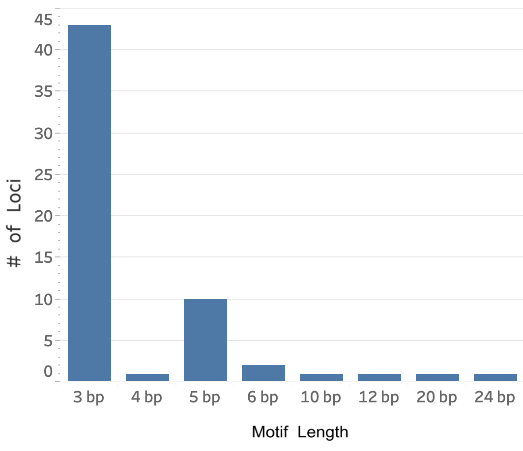
We ran ExpansionHunter [Dolzhenko 2019] on 18,511 whole genome samples from gnomAD v3.1 to generate calls for 60 disease associated repeat loci. These include 56 loci that have motifs between 3 and 6bp long and are traditionally called short tandem repeats (STRs), as well as 4 other loci with longer motifs of between 10 and 24bp. For brevity, we refer to all 60 loci as “STRs” below.

This minor release includes:

• Distributions of STR genotypes in the general population, with subsets by ancestry group and sex
• Visualizations of the read data for all samples at all 60 loci
• Collected reference information including disease associations and inheritance modes
• Downloadable variant catalogs for running ExpansionHunter on these 60 loci for either GRCh38 or GRCh37, with or without off-target regions
• A specialized approach for calling loci such as RFC1 where the pathogenic motif(s) differ from the motif in the reference genome
• Downloadable data table containing all results displayed in the browser, as well as additional results such as genotypes generated using off-target regions

These resources can be used as a comparison set for STR calls in rare disease cohorts, allowing users to see whether particular genotypes are common or rare. Additionally, we hope the provided variant catalogs and reference information will enable more researchers to genotype these loci in their own cohorts. Finally, the plots, read visualizations, and data file are designed to enable exploration of questions related to disease-associated STR loci.

Background

Short tandem repeats (STRs) are nucleotide sequences that consist of a short motif that repeats consecutively. For example, the HTT gene contains an STR locus at chr4:3074877-3074933 where the CAG motif (also known as the “repeat unit”) occurs 19 times. The human genome has millions of STR loci with various motifs. These loci can mutate through mechanisms such as strand slippage during replication, resulting in either an increase (i.e., expansion) or decrease (i.e., contraction) in the number of repeats. Collectively, STRs have a very high mutation rate, contributing approximately the same number of de novo mutations per generation as single nucleotide variants (SNVs), indels, and structural variants (SVs) combined ¹. During the last 30 years, approximately 60 STR loci have been identified as causal for monogenic diseases. In most cases, these loci cause disease only if they expand beyond a certain pathogenic threshold. For example, the CAG STR in the HTT gene causes Huntington Disease when it expands beyond 40 repeats. Some of the disease-associated STR loci also have an intermediate range below the pathogenic threshold that is associated with milder disease or reduced penetrance. For example, the intermediate range for HTT is between 36 and 40 CAG repeats. For some disease-associated loci such as RFC1 and DAB1, individuals may differ not only in the number of repeats, but also in the motif(s) that are present at the locus. Additionally, only a subset of these motifs may be disease-causing. For example, most individuals have AAAAG repeats within the RFC1 locus at chr4:39348425-39348479. However, some individuals have AAGGG repeats instead. Biallelic expansions of the AAGGG motif cause CANVAS, while expansions of the AAAAG motif do not cause disease.

Disease-Associated Loci

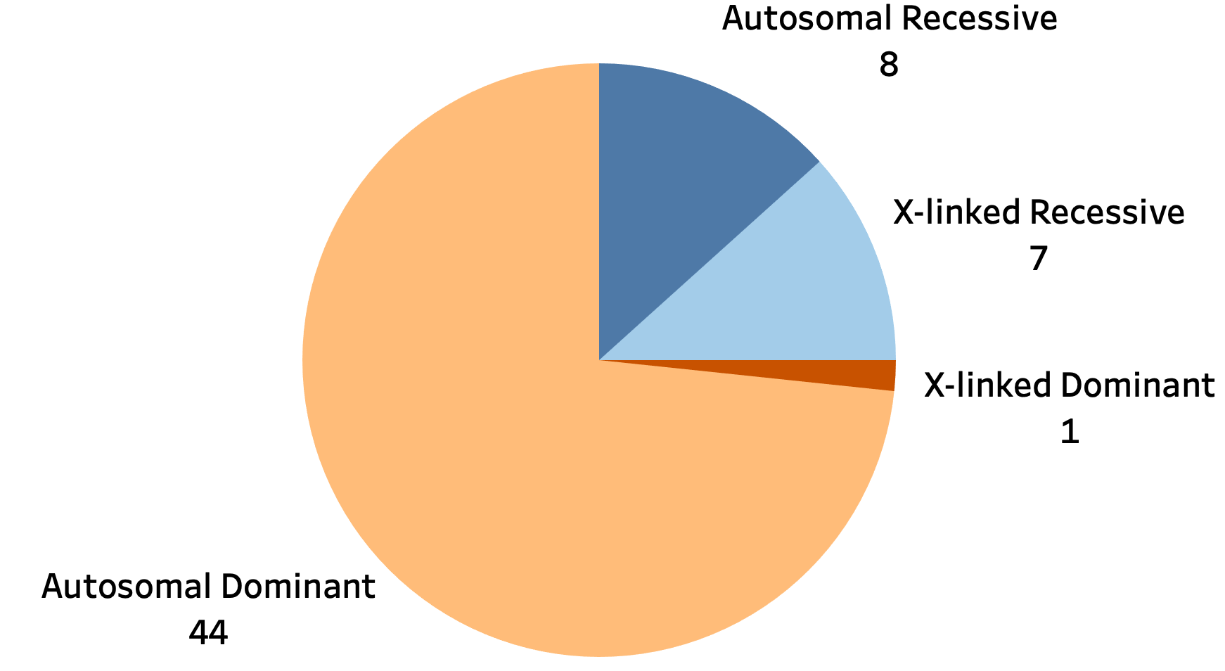
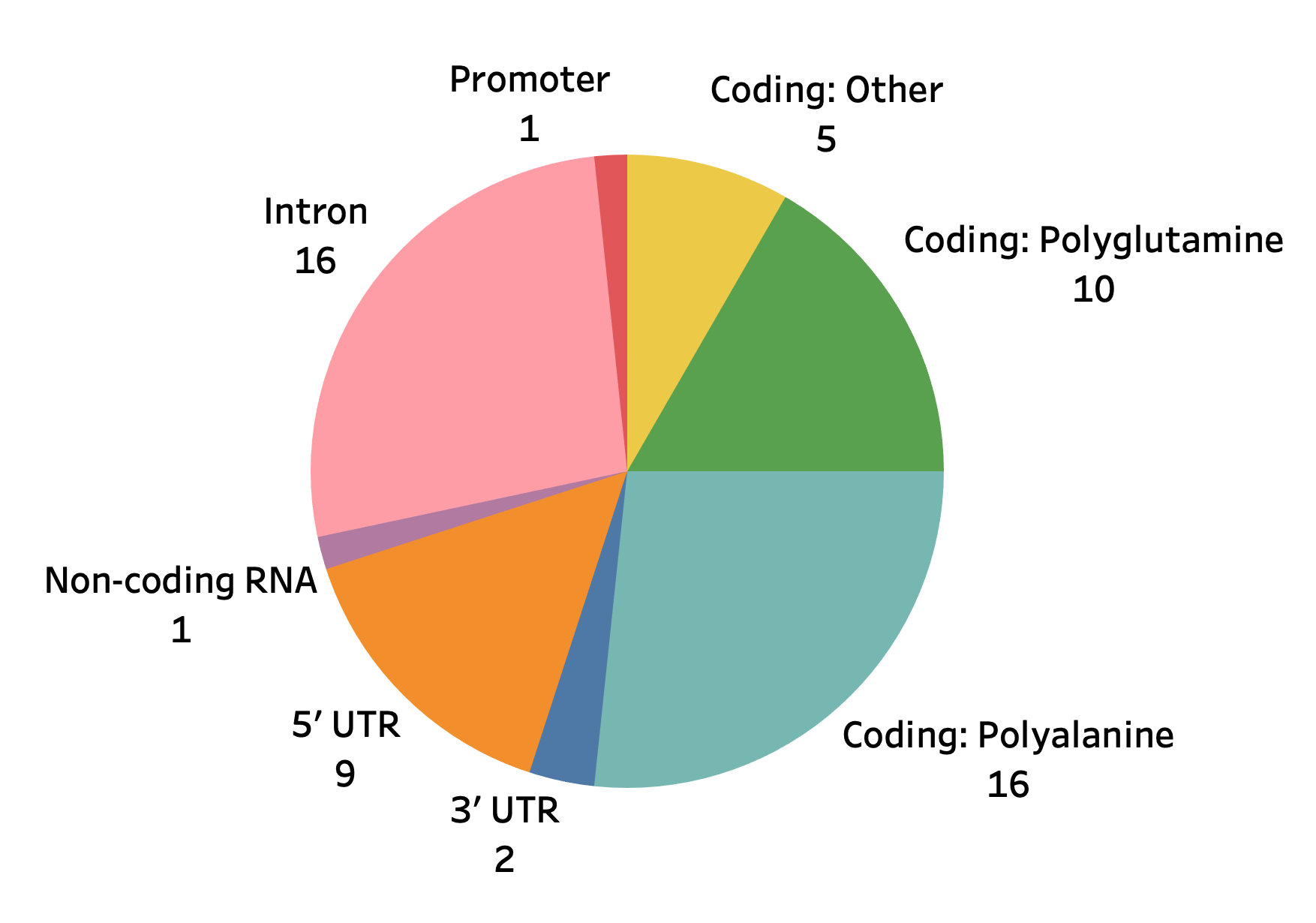
We collected and curated known pathogenic loci from sources such as [Depienne 2021], STRipy, OMIM, and GeneReviews. This yielded a catalog of 60 unique loci with the following characteristics:

Technical Details

To genotype the 60 disease-associated repeat loci, we chose to use ExpansionHunter [Dolzhenko 2017] because 1) we found that it had the best accuracy among existing tools for detecting expansions at disease-associated loci across a wide range of repeat sizes — both shorter and longer than read length, and 2) it’s now widely used for STR research and diagnosis in rare disease cohorts, including in [Ibanez 2020], [Stranneheim 2021], [van der Sanden 2021].

In order to run ExpansionHunter on these 60 loci, we generated an ExpansionHunter variant catalog that specifies the reference coordinates and motif of each locus.

We then ran an I/O-optimized version of ExpansionHunter v5 on the 18,511 gnomAD v3.1 samples for which the raw read data files were still available. We also ran REViewer to generate read visualizations for all samples at all 60 loci. Finally, we used python scripts in the STR-analysis repo to aggregate results and generate the STR data file available for download.

ExpansionHunter gives users the option to specify off-target regions which allow it to more accurately estimate large expansion sizes beyond fragment length (> ~350bp). However, off-target regions also increase the chance that ExpansionHunter will overestimate some genotypes. For more information about off-target regions, see [Dolzhenko 2017] and [Mousavi 2019]. In our experience with STR genotyping in rare disease cohorts, we have found that it is best to first run ExpansionHunter without off-target regions, even for loci such as DMPK or C9orf72 where we see very large expansions. Although this produces underestimated genotypes in some highly-expanded samples, these genotypes still turn out to be outliers relative to other individuals in the cohort, and can therefore be flagged and re-genotyped later using off-target regions. After considering the trade-offs, we chose to display only the results generated without using off-target regions. However, we provide results from running ExpansionHunter both with and without off-target regions in the downloadable data file. Additionally, we share two sets of variant catalogs — both with and without off-target regions.

The dataset includes 12,372 (64%) PCR-free samples, 2,423 (13%) PCR-plus samples and 4,446 (23%) samples with unknown PCR protocol. The per-sample PCR protocol information is displayed in the Read Data section of the STR pages and is also included in the STR data file available for download.

Loci with Non-Reference Pathogenic Motifs

Nine out of the 60 repeat loci are unusual in that they vary among individuals not just in the allele sizes, but also in the motifs present at the locus. These have been termed “replaced/nested” loci by [Halman 2021]. Existing STR genotyping tools such as ExpansionHunter and GangSTR require users to pre-specify the motif, and so do not work well for loci where the motif can vary. Other tools such as ExpansionHunterDenovo do not have this limitation, but typically cannot distinguish samples that carry two different motifs from samples with a single motif on both alleles. For example, for the RFC1 locus, the tools would have trouble distinguishing a sample that has a homozygous expansion of the AAGGG motif from a sample that has a short AAAAG repeat on one allele and a long AAGGG repeat on the other allele — a difference that is important for distinguishing carriers from affected individuals. As a temporary solution, we addressed these limitations by developing call_non_ref_pathogenic_motifs.py. This script first detects the one or two motifs present at each of these loci in a given individual and then runs ExpansionHunter for each motif to estimate its allele size as well as REViewer to generate read visualizations. The approach used by this script to detect motifs is, coincidentally, a simpler version of the approach used by the recently-released STRling tool. Unbiased comparisons are difficult given that we have a small number of positive controls and designed the script based on the positive controls we had available. However, we found that the script had slightly better sensitivity than STRling on positive RFC1 controls while maintaining high specificity. Additionally, it allowed us to generate read visualizations in a way not currently possible with other tools. A more detailed description of the script is available on GitHub and in a separate blog post.

Read Visualizations

We used the REViewer tool to generate read visualizations for all individuals at each locus. These images show the reads that ExpansionHunter considered when determining a genotype, and are primarily useful for identifying likely over-estimated genotypes and, to a lesser degree, under-estimated genotypes. We have included a section below, Supplemental Details for Examining Read Visualizations, that describes how to interpret these images.

Navigating STR Pages in the gnomAD Browser

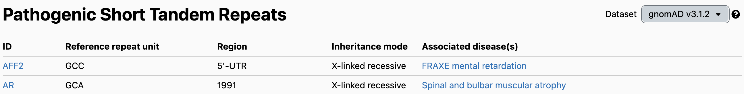
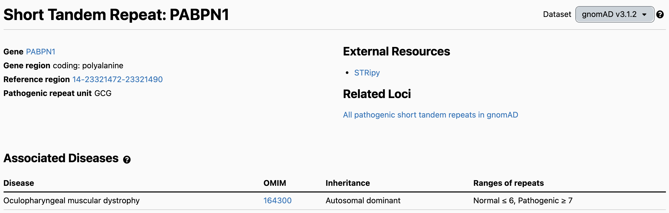
The STR table is the best place to start for exploring the STR data. It contains the list of 60 disease-associated loci, their repeat motif, genomic region, inheritance mode, and disease association(s).

As an example, we can look at the PABPN1 locus (chr14:23321473-23321490), which causes autosomal dominant oculopharyngeal muscular dystrophy (OPMD) when the number of GCG repeats expands to 7 or more on one allele. It should be noted that immediately to the right of the main GCG repeat sequence are 3 GCA repeats followed by a GCG. As GCA and GCG both code for alanine, early publications include these adjacent repeats in their definition of the locus, and therefore place the pathogenic threshold at  ≥ 11 repeats. Recent reviews such as [Depienne 2021] also use this definition. On the other hand, for technical reasons involving better ExpansionHunter accuracy on pure vs. non-pure repeats, we and others include only the 6 pure GCG repeats in our definition of the locus, and therefore define the pathogenic threshold as ≥ 7 repeats.

To see the PABPN1 STR page, we can scroll down in the table and click on “PABPN1”. Another option is to search the gnomAD browser for “PABPN1” and click on this note at the top of the PABPN1 gene page:

The STR page shows reference information about the locus and the associated disease, followed by the Allele Size Distribution. This histogram summarizes the numbers of GCG repeats found in gnomAD individuals. The y-axis represents alleles, so each individual contributes 2 counts to the distribution, except for STR loci on the X chromosome where male genotypes are hemizygous and thus contribute only 1 count.

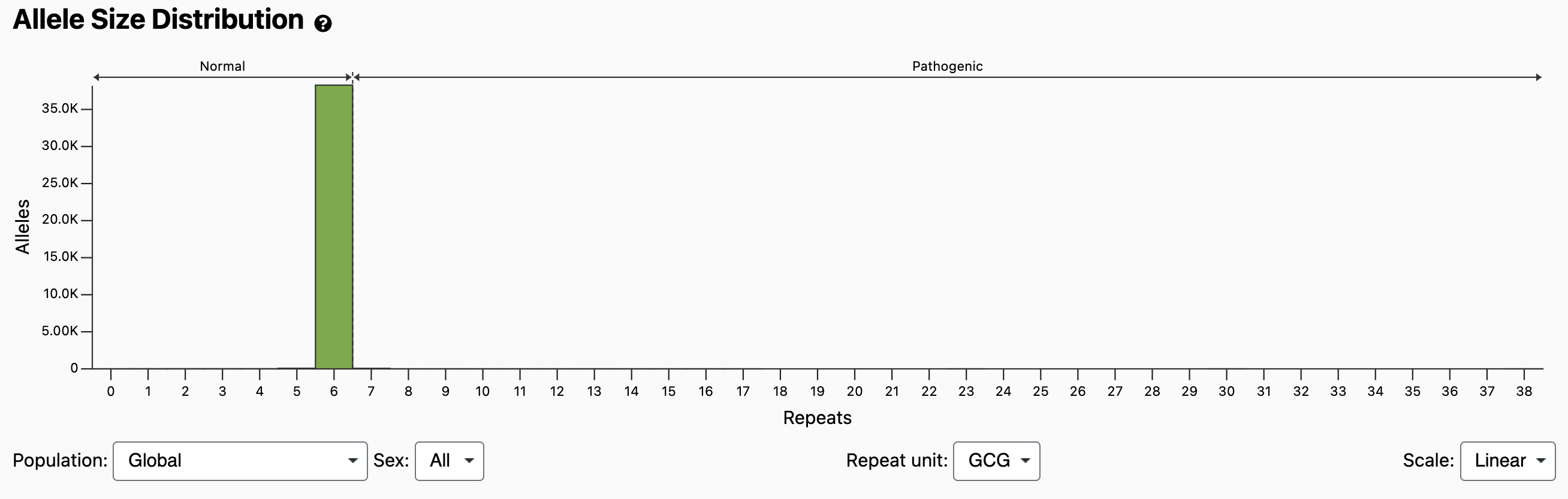
This distribution for the PABPN1 locus appears to show that all alleles are in the Normal range: ≤ 6 repeats. However, we can switch the scale from “Linear” to “Log” using the drop-down in the bottom right. This allows us to see the long tail of alleles with 7 or more repeats:

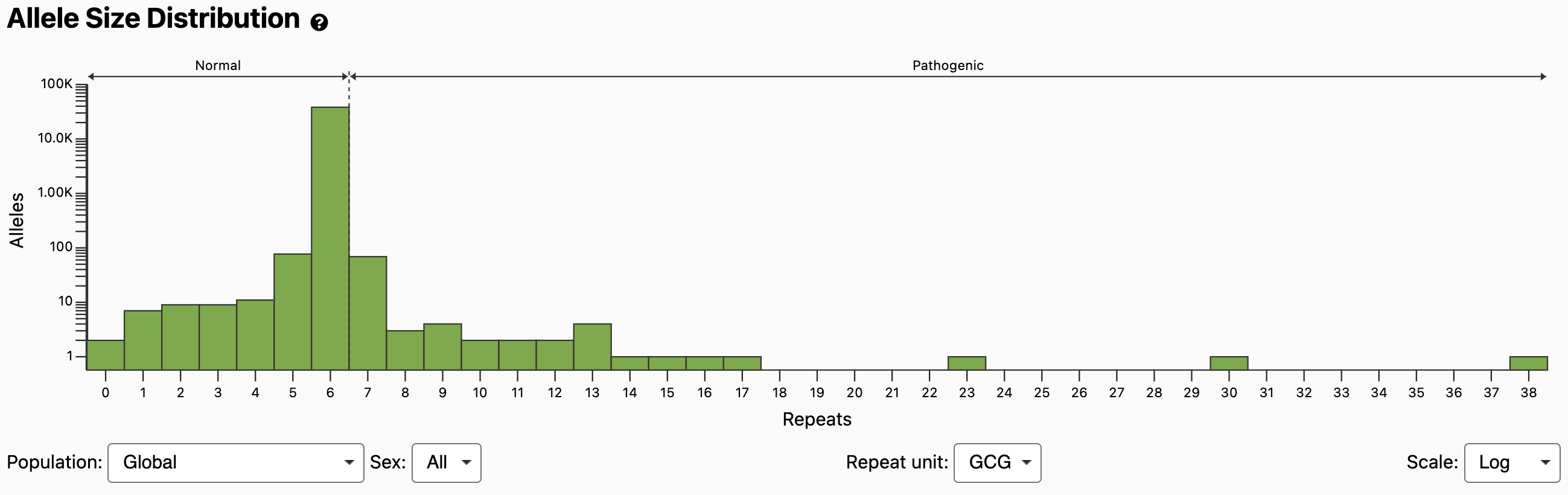
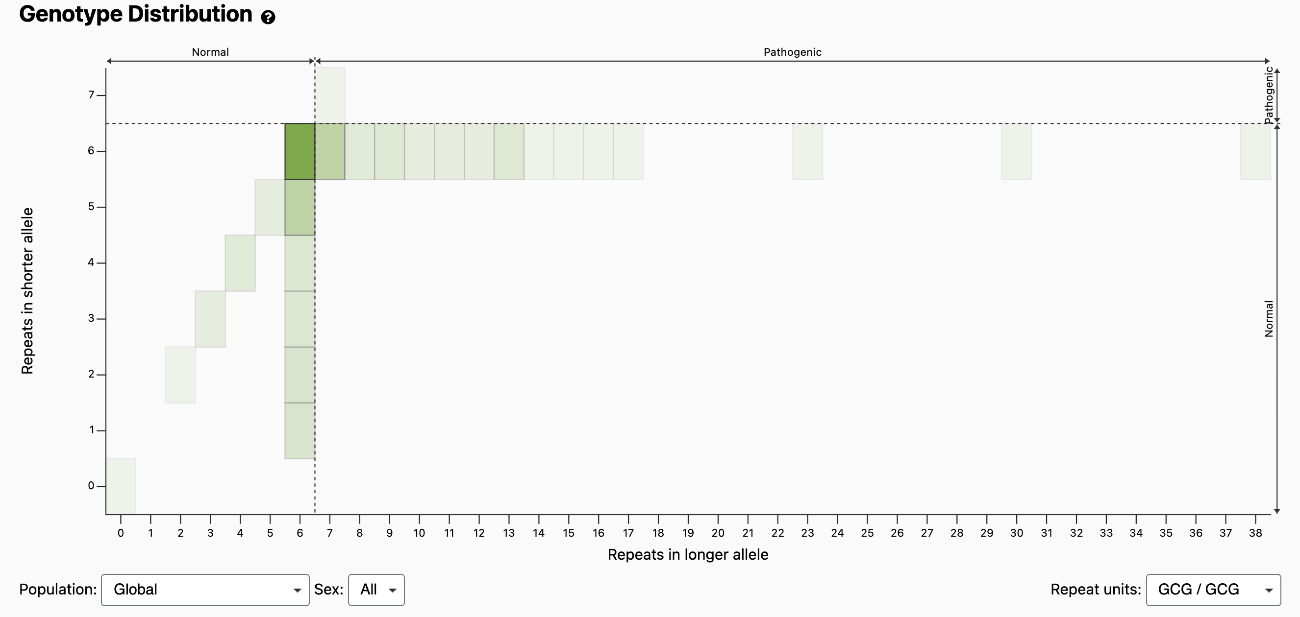
The normal and pathogenic ranges are indicated by horizontal arrows at the top of the plot, as well as by dashed vertical lines at the thresholds. It should be noted that compared with larger expansions, OPMD caused by 7 repeats has been shown to present with reduced  penetrance, later onset, or milder disease unless identified in homozygosity [Richard 2017]. Because the Allele Size Distribution counts each allele independently, it does not tell us diplotypes (e.g., how many individuals have a 6/7 compound heterozygous genotype vs a 7/7 homozygous genotype). However, if we scroll down to the Genotype Distribution and look at bin x=7, y=6, we see that it’s darker than the bin at x=7, y=7, which means more individuals have the 6/7 genotype. If we mouse over the bins, we can see the exact counts: 67 individuals have a 6/7 genotype and 1 individual has a 7/7 genotype.

Given that the prevalence of OMPD in the general population is estimated at 1 in 100,000, we expect to see fewer than 2 individuals in the pathogenic range, especially since the gnomAD dataset attempts to exclude cases with rare disease.

However, the typical age of onset for OPMD is 40 to 60 years old, so genotype positive individuals are less likely to be affected when recruited and therefore less likely to be excluded from gnomAD. If we scroll down to the Age Distribution, we see a plot where the y-axis represents age bins.

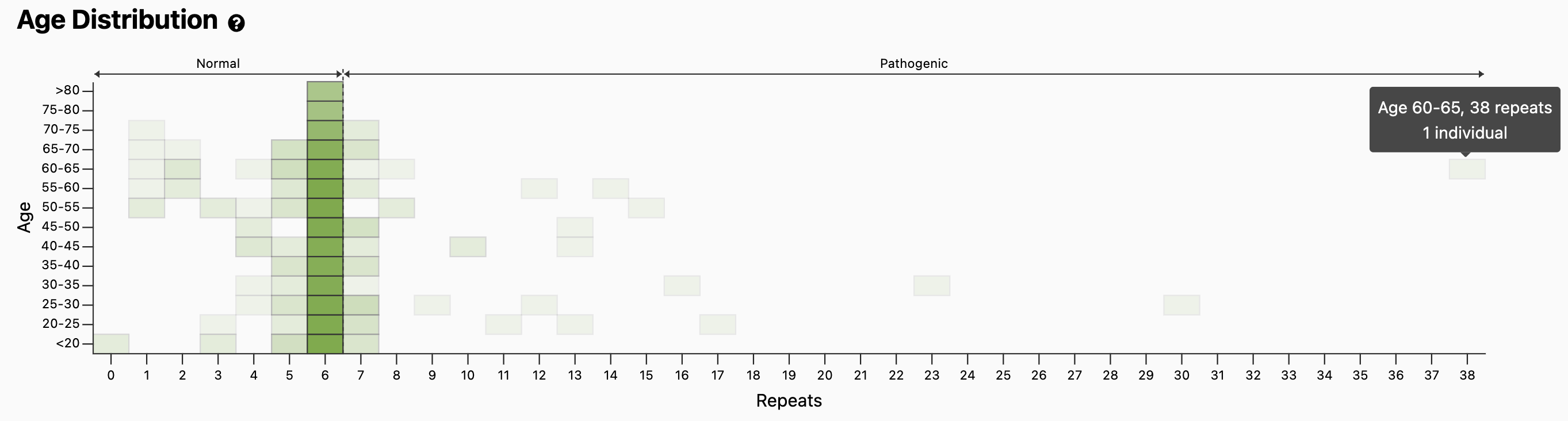
Mousing over the bins such as the one in the top-right shows several individuals of age 60-65yo, including the individual with 38 repeats, a genotype less likely to be present in the general population. However, one can evaluate the quality of the genotype data through read visualization.

To evaluate this, we can scroll down to the Read Data section and click the “Show read data” button. This displays the read visualization images, starting with the sample that has the longest expansion:

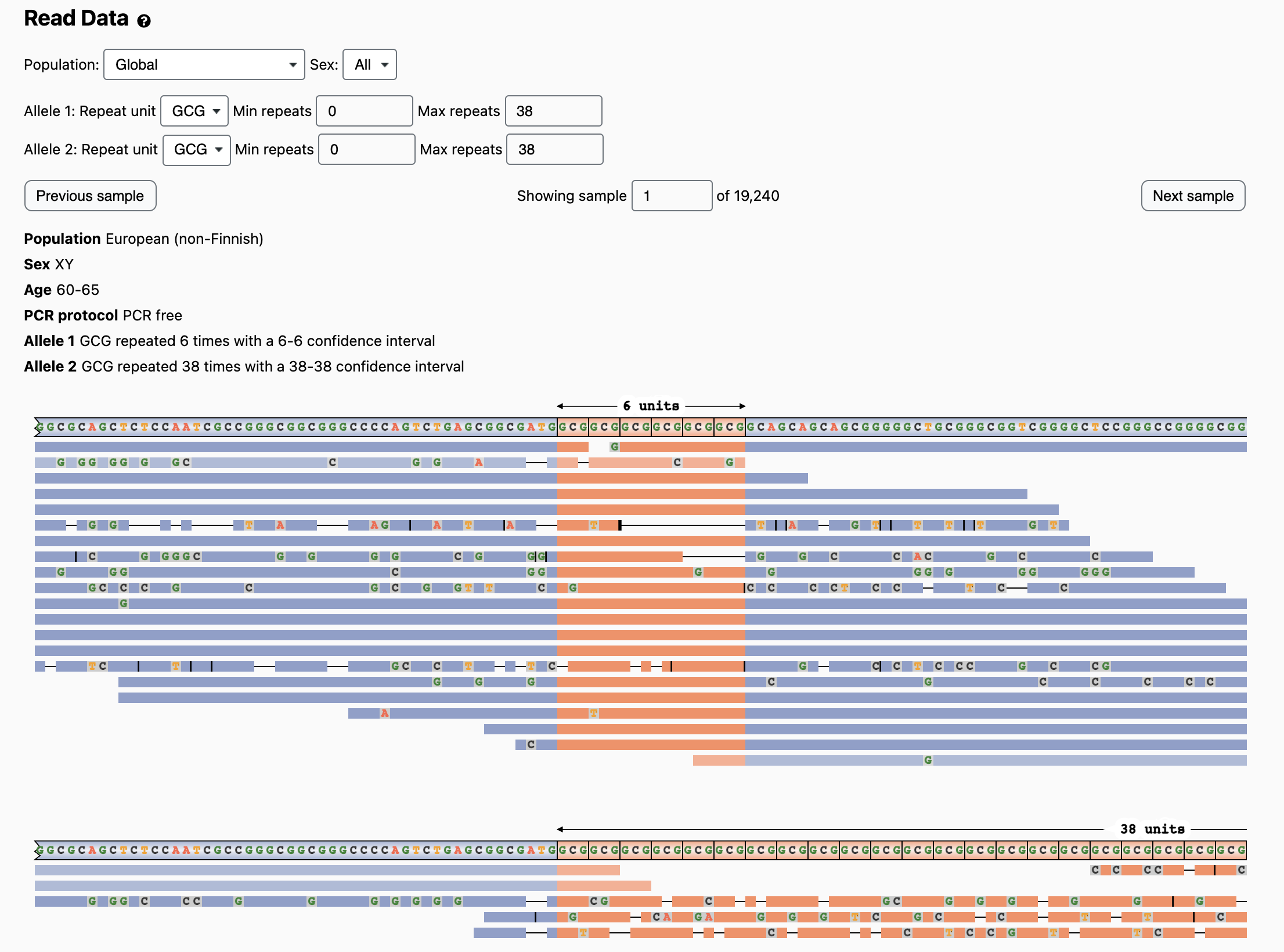
Users can click “Next Sample” and “Previous Sample” buttons to see more images generated by the REViewer tool for all individuals at this locus in order of expansion size. Another option is to first use the “Min repeats” or “Max repeats” filters and the Population and Sex filters to select individuals of interest. Above each image, users can see the population, sex, and age (if available) of the individual along with the ExpansionHunter genotype and confidence intervals for allele 1 and allele 2. Because some of the images are wider than the screen, users can scroll the image horizontally or right-click and select “Open Image in New Tab” to see the full image.

Looking at the reads supporting the pathogenic PABPN1 genotypes, we see that the first image is from the individual with the 6/38 genotype. It has two sections: the top section shows reads that support the short allele, and the bottom section shows reads that support the long allele. Here we see multiple deletions in both the repeat sequence (orange) and flanking regions (blue):

This suggests that most or all reads supporting the long allele are misaligned, and that the genotype is very likely to be incorrect (see Supplemental Details for more information).

Clicking the “Next Sample” button, we see subsequent samples also have questionable alignments underlying their long allele sizes. In some cases, the reads are full of mismatches rather than deletions, but the conclusion is the same. By reviewing these images, we find that all alleles > 9 repeats are likely to be technical artifacts. Only when we reach the 6/9 genotypes do we find several well supported 9-repeat alleles with multiple spanning read alignments that lack mismatches or indels:

The age of one of these 6/9 individuals is 25-30 years old. However, there is also a high quality 6/8 genotype in a European individual with age 60-65.

In summary, these read visualizations suggest that many pathogenic-range PABPN1 alleles with lengths beyond 7 repeats are technical artifacts. They also highlight some challenges in interpreting STR calls and the importance of validating genotype calls.

Discussion

Tools to automatically filter ExpansionHunter genotypes are needed, and are an active research area. Additionally, a full understanding of pathogenic thresholds and disease penetrance at different repeat sizes and in different populations is still lacking for most loci.

Although we have collected normal and pathogenic thresholds from different reference sources and provide them in the browser, these thresholds should be treated as approximate. Even for loci with long-established disease associations, it can be difficult to draw exact lines separating normal, intermediate, and pathogenic genotypes due to the variability in disease phenotypes across individuals and populations, and ambiguity in STR locus boundaries.

Overall, we expect pathogenic thresholds and other reference information to continue to undergo revisions as STR research continues.

We hope that this release of the STR callset browser and data files will contribute to the study of STR variation and assist with using WGS for the diagnosis of STR disorders. We encourage users to write to gnomad@broadinstitute.org with any questions or comments.

Acknowledgments

We thank Nehir Kurtas and Stephanie DiTroia for helping to curate the list of disease-associated STR loci and reviewing the literature on pathogenic alleles; Katherine Chao for suggestions and code reviews; Egor Dolzhenko for consultations on ExpansionHunter, REViewer, and other topics; Depienne et al. and Halman et al. authors for publishing these very useful resources; Yossi Farjoun for mentorship during the initial stages of the project; Jackie Goldstein, Daniel King, Cotton Seed and the rest of the Hail team for building Hail Batch and other tools that simplified the process of generating this dataset.

Supplemental Details for Examining Read Visualizations

Below we describe visual features of REViewer images and show how these can be used to identify overestimated or underestimated genotypes:

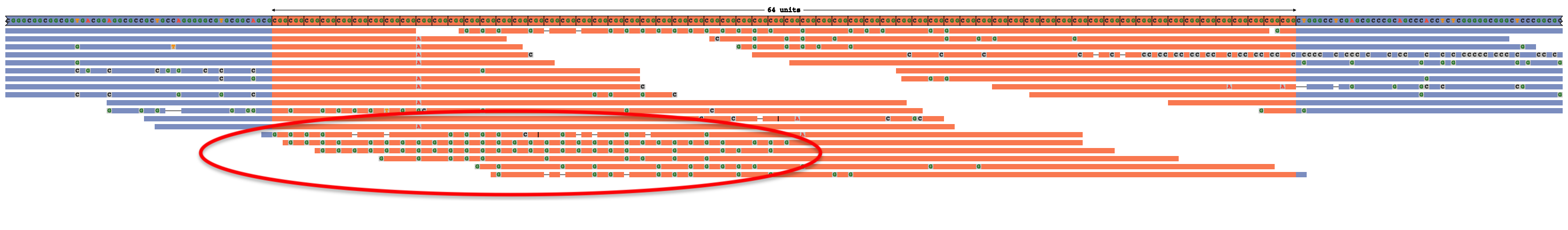
▪ Deletion(s) within a read are shown as gaps: . Multiple deletions within a read may indicate an erroneous alignment and raise the chances of this being an overestimated expansion size. For example, the true genotype here is 51 x CGG rather than 64 x CGG, and multiple deletions in reads that are located entirely within the repeat sequence (along with the G mismatches in their left halves) suggest that these reads are misaligned [full image]:

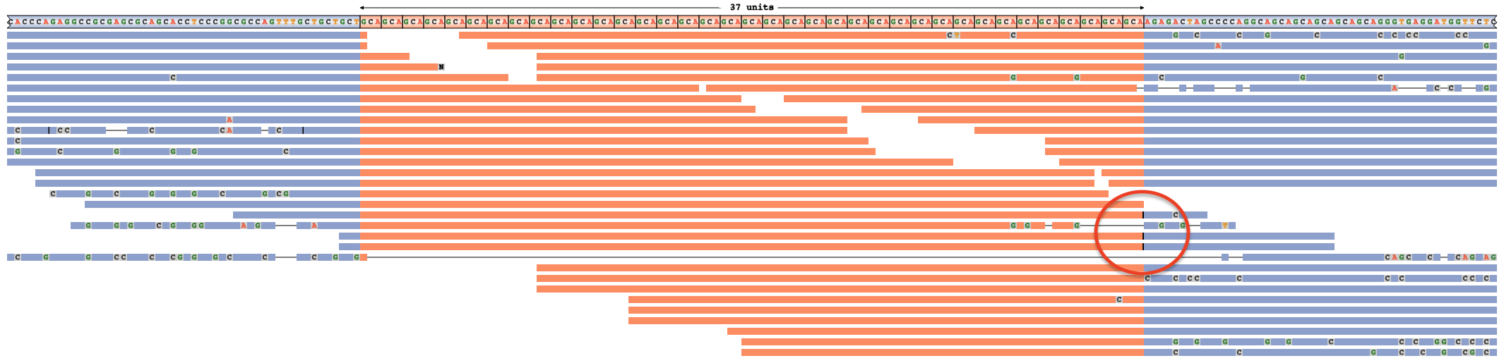
▪ Insertion(s) within a read are shown as vertical black bars (analogous to the purple bar in IGV): . When many reads contain insertions beyond the already plotted sequence, this raises the chances that the expansion size has been underestimated. For example, the true genotype below is 42 x GCA instead of 40 x CAG. All three spanning reads hint at this, due to insertions between their repetitive (orange) and right flanking (blue) regions — annotated with a red circle [full image]:

▪ When all except one or two reads support a shorter genotype, there’s an increased chance the expansion size is overestimated. For example, the true genotype here is 22/22 x CAG instead of 22/42 [full image]. The single read supporting a 42 repeat genotype is annotated with a red circle below:

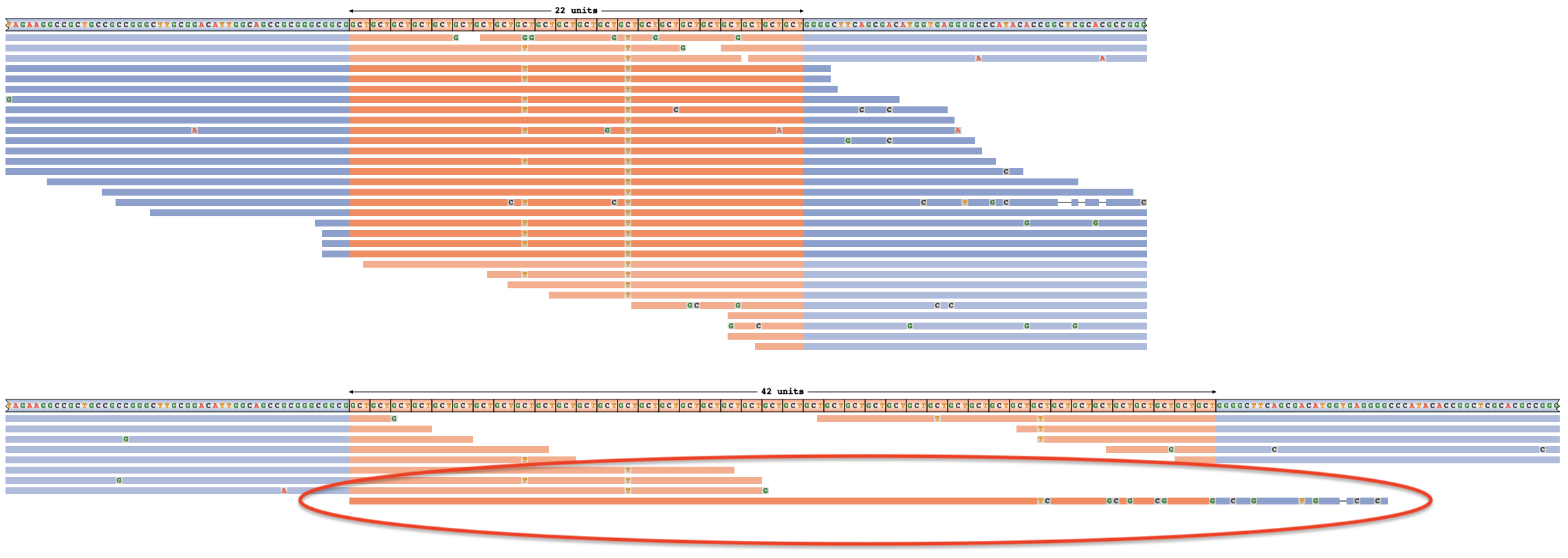
▪ The darker-color and lighter-color shading of reads in the example above distinguishes reads that only support one of the two allele sizes (dark color) vs reads that equally support both allele sizes (light color). In the example above, the reads with shorter repetitive regions are consistent with either the 22 repeat allele, or the 42 repeats, further highlighting that the long allele size estimate rests on evidence from only one read.

▪ Mismatches with the reference (eg. SNVs) appear as letters within reads: . These are useful for exploring STR interruptions and as additional indicators of the true expansion size. In the previous example, lining up the “T” interruptions in the left-flanking reads with the “T” interruptions in the right-flanking reads suggests the correct 22 x CAG genotype instead of 42 x CAG.

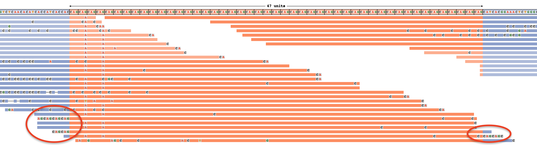
▪ Soft-clipped bases appear at the beginning or end of a read and represent bases that the aligner considered to be unaligned. They appear as a string of mismatches at the end of a read (like in IGV): . As with deletions, the presence of soft-clipped bases may indicate poor quality alignments and therefore point to an overestimated expansion size. However, in some cases they may suggest an underestimate instead. For example, the three reads showing additional CAGs in their soft-clipped bases below hint that the true genotype may be longer than 47 x CAG. Indeed, PCR confirmed the true genotype to be 54 x CAG in this sample [full image]:

July 2022 Update:

• Removed 732 samples with 100bp read lengths which were inadvertently included in the initial release and kept only the 18,511 samples that have 150bp read lengths.
• Added data for the RILPL1 locus which was recently published as associated with oculopharyngodistal myopathy type 4 (OPDM) [Yu 2022].