We’re proud to announce the gnomAD v3.1 release of 759,302,267 short nuclear variants (644,267,978 passing variant quality filters) observed in 76,156 genome samples.
In this release, we have included more than 3,000 new samples specifically chosen to increase the ancestral diversity of the resource. As a result, this is the first release for which we have a designated population label for samples of Middle Eastern ancestry, and we are thrilled to be able to include these in the following population breakdown for the v3.1 release:
| Population | Description | Genomes |
|---|---|---|
| afr | African/African American | 20,744 |
| ami | Amish | 456 |
| amr | Latino/Admixed American | 7,647 |
| asj | Ashkenazi Jewish | 1,736 |
| eas | East Asian | 2,604 |
| fin | Finnish | 5,316 |
| nfe | Non-Finnish European | 34,029 |
| mid | Middle Eastern | 158 |
| sas | South Asian | 2,419 |
| oth | Other (population not assigned) | 1,047 |
Topics
The changes and new features in this release include:
- Innovation in incremental joint calling
- Documentation of functions and code used to generate the callset
- Individual-level genotypes available for HGDP + 1KG subsets
- Read visualizations in noncoding regions
- New subset availability for frequency annotations
- New in-silico prediction annotations
- Tweaks and updates to VEP, dbSNP rsIDs, homozygous genotypes in common variants, and terminology for individuals’ chromosomal sex
- Fully free access to downloadable datasets on multiple cloud providers
We’ll discuss each of these features in greater detail in the sections below and, at the end, we’ll share updated plots for v3.1 sample and variant QC.
Incremental joint-calling
To create gnomAD v3, the first version of this genome release, we took advantage of a new sparse (but lossless) data format developed by Chris Vittal and Cotton Seed on the Hail team to store individual genotypes in a fraction of the space required by traditional VCFs. In a previous blog post describing this innovation, we noted that one advantage of this new format was the possibility of appending new data to existing callsets without needing to re-process samples already joint called as part of prior gnomAD releases—effectively solving the “N+1” joint calling problem.
For gnomAD v3.1, we made good on this promise, adding 4,598 new genomes in gVCF form to the already extant, joint-called gnomAD v3 callset stored in the sparse Hail Matrix Table format. This is, to our knowledge, the first time that this procedure has been done. Chris Vittal added the new genomes for us in six hours—shaving off almost a week of compute time (or several million core hours) that would have been required if we had created the callset from scratch.
The total cost of the addition was about $400, or ~$0.09 per new sample and ~$0.004 per existing sample. By contrast, creating the callset from scratch would have cost ~$13,000.
The gnomAD Python package
Over the last year, we’ve collectively poured thousands of hours into curating and fully documenting a public code repository with Python functions we repeatedly use to produce large callsets, including but not limited to gnomAD. The gnomAD v3.1 production pipeline drew heavily on this resource, and we hope that others will benefit from it as well.
The package includes functions to help users handle sparse Matrix Tables, annotate variants with VEP, lift over sites from GRCh37 to GRCh38 (or vice versa), infer ancestry and cryptic relatedness within a callset, infer chromosomal sex, train and evaluate random forests variant filtering models, interact with linkage disequilibrium Block Matrices, export data to standard VCF format, and much more.
Users can access the entire repository with a simple command:
$ pip install gnomad
The gnomAD HGDP and 1000 Genomes callset
We’re delighted to provide, for the first time, downloads with individual-level genotypes for a subset of gnomAD that is available to the public with no access restrictions. We hope this resource will be useful for a broad range of research applications — serving as a diverse reference panel for haplotype phasing and genotype imputation, for example, or as a training set for ancestry inference.
The samples included in this subset are drawn from the 1000 Genomes Project (n=2,500) and the Human Genome Diversity Project (n=780), which contain some of the most genetically diverse populations present in gnomAD. Collectively they represent human genetic diversity sampled across >60 distinct populations from Africa, Europe, the Middle East, South and Central and South Asia, East Asia, Oceania, and the Americas.
To create this callset, we re-processed raw data from the 1000 Genomes Project and HGDP to meet the functional equivalence standard and joint-called the re-processed data with the rest of the gnomAD callset. (See “Incremental joint calling” above for more details on the joint-calling process.) The callset contains all high-quality samples (n=3,942) from these projects that passed gnomAD sample QC filters. These files therefore contain data for individuals (n=662) that we did not ultimately include in the gnomAD v3.1 aggregate allele frequencies, as these individuals were found to be second-degree related (or closer) to other individuals in 1000 Genomes, HGDP, or the larger gnomAD callset. We have provided a sample metadata table containing each sample’s status of inclusion or exclusion in the v3.1 release, along with sample-level quality control metrics and ancestry labels to accompany the VCF. (This information is directly annotated as column annotations in the Matrix Table version of the callset.)
All variants found in this cohort of samples are included, along with the variant filter status, metrics used to assess variant quality, and gnomAD v3.1 allele frequencies.
All called genotypes are included in this dataset, including low-quality genotypes that we filtered before computing gnomAD allele counts, allele numbers, and allele frequencies. To reproduce gnomAD genotype filtering, users should filter to genotypes with genotype quality (GQ) >= 20, depth (DP) >=10 (5 for haploid genotypes on sex chromosomes), and allele balance (AB) >= 0.2 and <= 0.8 (for heterozygous genotypes only). Users working with the Matrix Table version of the dataset can call the annotate_adj() function in the gnomAD Python package to annotate and filter genotypes:
$ mt = annotate_adj(mt)
$ mt = mt.filter_entries(mt.adj)
The code above adds an adj (“adjusted,” or passing) genotype annotation using the default gnomAD thresholds and then removes any genotype whose adj status is False.
Read visualizations for non-coding regions
Since our beginning as a project, we’ve made read data visualizations available for representative genotypes for most of the variants we observe in gnomAD exome data. Generating read visualizations for v3.1 whole genome data, however, has been considerably more challenging, as 99% of the genome is non-coding: there’s a lot more genomic territory to cover in whole-genome data.
Consider the following numbers: to support non-coding read visualizations in this release, we generated over 2.5 billion read visualizations representing nearly 600 million unique variants observed in gnomAD v3.1. To be exact, we collected reads for 2,573,960,015 non-reference genotypes observed across 584,562,724 unique variants.
We needed a creative approach to generate, store, and serve up this data efficiently on the browser. Ben Weisburd on our team conceived a process that allowed us to extract reads for multiple variants from each individual sample, thus producing an individual mini-BAM—a file containing all the sequencing reads aligning to a specified list of variants in a given individual—for each available sample in gnomAD. (Not all samples in gnomAD had available read data, which is why some variants in v3.1 are missing read visualizations.)
He then combined these individual mini-BAMs into composite, multi-sample mini-BAMs comprised of data from 50 individuals each; replaced the original read group tags with hashes to anonymize the combined data; and recorded which genotypes and loci were covered in each 50-sample composite file. (Read group tags were replaced as a precaution against re-identification of individuals included in each multi-sample mini-BAM: read group tags, which are assigned to a given sequencing run, might otherwise be used to re-link genotypes across the genome for a specific individual. After replacing tags with hashes, the genotype data stored in a composite mini-BAM is completely unlinked to individuals.)
The browser queries a database that contains an index of genotype hashes, loci, and composite filepaths: each time you pull up a variant page with available read visualizations, the browser queries this database to discover which composite file to load into IGV and which unique read group hash to use to extract the reads specific to the genotype you’re viewing.
With this carefully engineered system in place, we’re excited to make read data visualizations for non-coding variants available for the very first time.
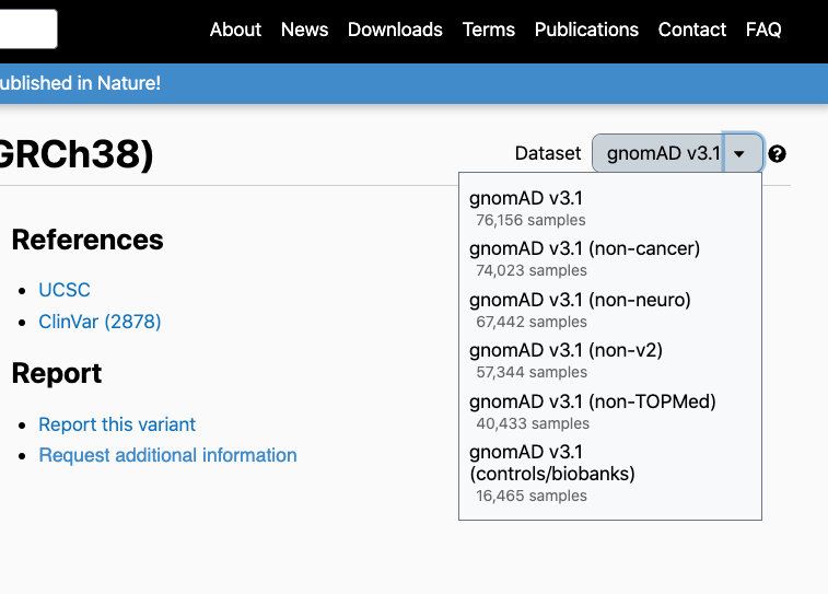
Subsets
By popular request, we’ve computed allele counts and allele frequencies for major subsets of gnomAD v3.1, as follows:
- Non-v2: only genome samples that are new to the v3 or v3.1 release and not included in the v2 genomes
- Non-TOPMed: only samples that are not present in the Trans-Omics for Precision Medicine (TOPMed)/BRAVO release. The allele counts in this subset can thus be added to those of BRAVO to enable federated use of both datasets
- Non-cancer: only samples from individuals who were not ascertained for having cancer in a cancer study
- Controls and biobanks: only samples collected specifically as controls for disease studies, or samples belonging to biobanks (e.g. BioMe, Genizon) or general population studies (e.g., 1000 Genomes, HGDP, PAGE)
- Non-neuro: only samples that were not collected as part of a neurologic or psychiatric case/control study, or samples collected as part of a neurologic or psychiatric case/control study but designated as controls
Subset-specific allele counts and allele frequencies are available on variant pages by clicking on the drop-down menu at the top-right corner of the page:
Viewers will note that in addition to the gnomAD population frequencies, population frequencies specific to the HGDP and 1000 Genomes cohorts are available:
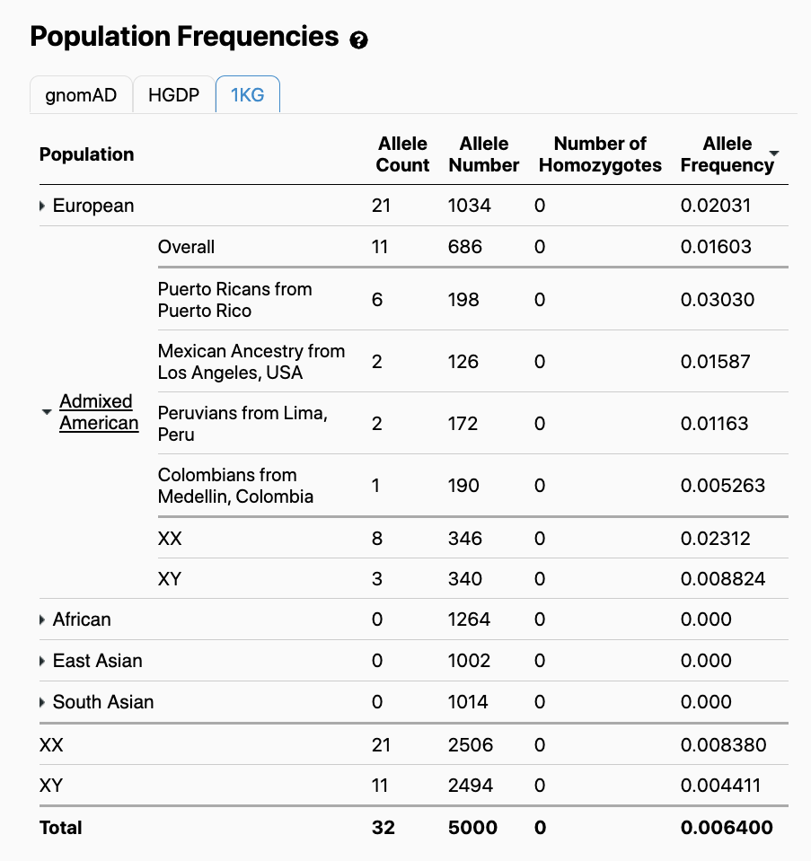
We provided allele counts and population frequencies for HGDP and 1000 Genomes to allow users to observe and compare the distribution of variant alleles across a diverse range of distinct human populations.
In-silico prediction annotations
We have added a number of variant annotations to help users interpret the clinical and functional effects of variants without needing to navigate to other websites and databases:
- REVEL, an ensemble score for predicting the pathogenicity of missense variants (based on 13 other variant predictors)
- CADD v1.6, a score predicting deleteriousness for both SNVs and indels
- SpliceAI, an deep learning predictor for variant effects on splicing
- PrimateAI, a deep neural network-trained score for classifying pathogenicity of missense mutations
We would particularly like to thank Kishore Jaganathan and Kyle Farh at Illumina for their material assistance in generating SpliceAI annotations for v3.1 variants.
Tweaks and updates
This latest release uses an updated version (v101) of the Variant Effect Predictor (VEP) based on the most recent Gencode v35 gene models to provide consequence annotations. We have also updated the dbSNP release (b154) we use to annotate reference SNP identification (rsID) numbers. Users have alerted us to occasional rsID annotation errors in previous releases, which were caused by our pipeline matching rsIDs by chromosomal locus only. We now annotate rsIDs using both locus and allele information, which should reduce errors and ambiguities in annotation.
Another error mode identified in our previous releases is a technical artifact wherein homozygous alternate genotypes (particularly at long indel sites) were called as heterozygous genotypes despite having very high allele balances characteristic of homozygous alternate genotypes. This problem, described in greater detail here, is caused by sample contamination, which can introduce stray reads supporting a reference allele at a site where the majority of reads contain an alternate allele. The genotype likelihood model used by our variant caller (GATK HaplotypeCaller) did not handle this condition properly.
The issue is now fixed for new gVCFs generated by HaplotypeCaller moving forward. However, for this release, the majority of variant calls were already generated using an uncorrected version of HaplotypeCaller. We therefore made an adjustment to heterozygous genotypes with highly skewed allele balance (>0.9) at common variant sites (>0.01 AF), setting these genotypes to homozygous alternate genotypes. This change is reflected in the aggregate allele frequencies, allele numbers, and allele counts displayed on the browser as well as in the genotype data released for the gnomAD HGDP and 1000 Genomes callset.
Finally, we have changed the labels we use to classify individuals by chromosomal sex from “male” and “female” to “XY” and “XX,” respectively. While we have always used the terms “male” and “female” to refer to an individual’s chromosomal sex and not to gender, we recognize that this terminology is overloaded and could cause confusion to users. We also note that the terms “male” and “female,” when referring to chromosomal sex, can be applied to individuals with sex chromosomal aneuploidies, such as 47,XYY or 45,X. Since we remove samples with sex chromosomal aneuploidies from gnomAD during the QC process, we felt the most straightforward sex classification labels were “XX” and “XY.” This change is now reflected in both the v3.1 download files and in the browser.
Free data access on multiple cloud providers
One recent development we’re excited to share with users is the availability of all gnomAD data on three cloud providers: Amazon Web Services, Microsoft Azure, and Google Cloud. All VCFs and Hail Tables from each gnomAD release are now available to download or read for free from each of these providers. Working in partnership with their public data hosting programs, we hope to encourage an even wider range of individuals and institutions to make use of gnomAD data for innovative research in human genetics and for the development of translational tools and medicines to treat and cure disease. For more details on how to access gnomAD through these cloud providers, read our blog post here.
Sample and variant quality control
The overall approach to both sample and variant QC were very similar to the methods used for QC of gnomAD v3.
Sample QC hard filtering
Sample QC metrics were computed using Hail’s sample_qc() module on all autosomal bi-allelic SNVs, and outliers were filtered using the following cutoffs:
- Number of SNVs: < 2.4M or > 3.75M
- Number of singletons: > 100k
- Ratio of heterozygous to homozygous variants: > 3.3
Hard filtering using BAM-level metrics was performed when such metrics were available. We removed samples that were outliers for:
- Contamination: > 5%
- Chimeras: > 5%
- Median insert size: < 250
Additionally, samples were filtered if they had a mean coverage on chromosome 20 < 15X.
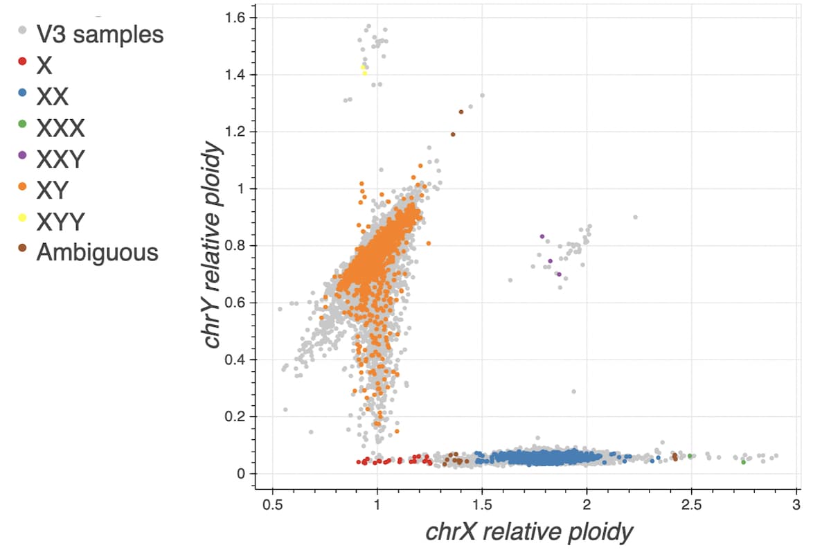
Sex inference
The process of imputing sex was the same as the method used for gnomAD v3, with slightly modified cutoffs. In previous releases, we used cutoffs on F-stat to determine XX and XY. The current pipeline uses a rough F-stat cutoff of 0.5 to split samples into the XX and XY categories. The final X and Y ploidy cutoffs are then determined from the means and standard deviations of those XX and XY distributions. Sex was assigned based on the following cutoffs:
-
XY:
- normalized X coverage < 1.29 &
- normalized Y coverage > 0.1 &
- normalized Y coverage < 1.16
-
XX:
- normalized X coverage > 1.45 &
- normalized X coverage < 2.4 &
- normalized Y coverage < 0.1
The plot below overlays the new v3.1 samples onto the normalized X coverage vs. normalized Y coverage plot with gnomAD v3 samples displayed in grey.
Ancestry inference
The method for ancestry assignment was similar to the method used for v3, with some slight changes in parameters and evaluation. 30 principal components (PCs) were computed using principal components analysis (PCA) as implemented by the hwe_normalized_pca() Hail function on 76,419 high-quality variants selected as follows:
- We took all sites that were used for gnomAD v2.1 and lifted them over to GRCh38
- We added ~5k sites widely used for quality control of GWAS data defined by Shaun Purcell and lifted these sites over to GRCh38
- From these two sets of sites, we then selected all bi-allelic SNVs with an Inbreeding coefficient > -0.25 (no excess of heterozygotes)
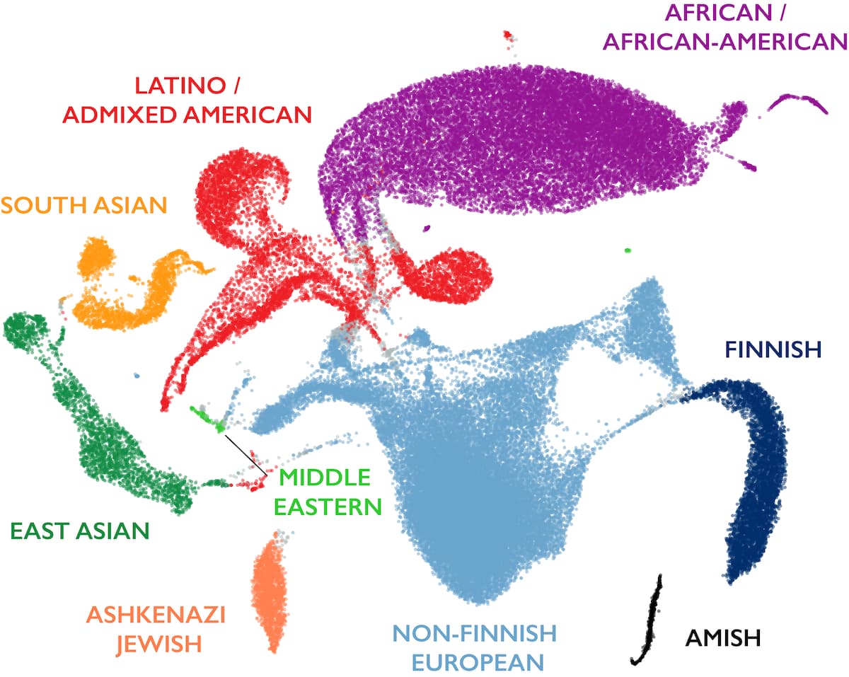
The 30 PCs were visually inspected to determine which PCs were capturing variance explained by available ”known” population labels, which are obtained from a variety of sources, including labels captured by prior research studies as well as individual self-reported population labels. We determined that the first 16 PCs captured global ancestry variation with a clear drop in information content for higher PCs. We then trained a random forests classifier using those first 16 PCs as features on the samples with “known” population labels. Many of the new samples in v3.1 had “known” population labels, increasing the total samples used for training from 32,955 in v3 to 36,882 for this release. Ancestry labels were then assigned to all samples for which the random forest probability of that population assignment was > 75% according to the random forests model, and all remaining samples were given a population label of “other” (oth). The 75% cutoff was determined by holding back 20% of the samples with “known” population labels for evaluation of the model. We want to expressly acknowledge that this method of global ancestry assignment using self-reported population labels as a training set does not account for differences between genetic ancestry and self-reported population labels that are known to exist.
The figure below shows a 2D uniform manifold approximation and projection (UMAP) of ancestry principal components 1-6 and 8-16, colored by the inferred ancestries of the samples. Note that long-range distances in this projection do not reflect genetic distance between populations.
Sample QC metric outlier filtering
As with gnomAD v3, we used the approach of determining sample QC outliers by computing sample QC metrics using the Hail sample_qc() module and regressing out the first 8 ancestry assignment PCs. Then we filtered samples that fell outside 4 median absolute deviations (MADs) from the median for the following metrics: n_snp, r_ti_tv, r_insertion_deletion, n_insertion, n_deletion, n_het, n_hom_var, n_transition, and n_transversion. Additionally, we filtered samples over 8 MADs above the median n_singleton metric and over 4 MADs above the median r_het_hom_var metric.
Variant QC
As with gnomAD v3, we performed variant QC using the allele-specific version of GATK Variant Quality Score Recalibration (VQSR) with the following features:
- SNVs:
AS_FS,AS_SOR,AS_ReadPosRankSum,AS_MQRankSum,AS_QD,AS_MQ - Indels:
AS_FS,AS_SOR,AS_ReadPosRankSum,AS_MQRankSum,AS_QD
We used the standard GATK training resources (HapMap, Omni, 1000 Genomes, Mills indels) in addition to ~19M transmitted singletons (alleles confidently observed exactly twice in gnomAD, once in a parent and once in a child) from 6,743 trios present in the raw data.
The figure below shows the precision and recall curves for the allele-specific VQSR model (AS_VQSR_TS) using a truth sample (NA12878) present in our data. The lines at 90 (SNVs) and 80 (indels) indicate the cutoffs we chose for filtering.
 The same variant hard filters were applied:
- No high-quality genotype (GQ>=20, DP>=10, and AB>=0.2 for heterozygotes) called for the variant
- InbreedingCoeff < -0.3
These filtering criteria excluded 12.2% of SNVs and 32.5% of indels, resulting in 569,860,911 SNVs and 74,407,067 indels that passed all filters in the v3.1 release.
Updates:
- August 14, 2023 to correct the number of 1000 Genomes Project samples from 2,435 to 2,500.
- December 17, 2021 to provide additional details to the ancestry inference section of this post.